Paper Summary for Recursive Looped Transformers: Parameter Efficiency
Published:
This blog is also available in Chinese version: https://zhuanlan.zhihu.com/p/1962483093102400303
Loops and recursion have always been important techniques in deep learning. For example, the well-known Recurrent Neural Networks (RNN), compared to traditional neural networks, have the advantage of being able to pass information across time dimensions through hidden states, enabling models to capture temporal dependencies in context. In the era of large language models, researchers have further explored what role loop and recursion mechanisms can play in today’s increasingly Large Language Models. While Scaling Laws tell us that the final performance of large language models is closely related to their parameter count and the amount of training corpus, at the same time, recursive strategies can also play an important role in LLM scenarios.
Recent articles about applying recursive mechanisms in LLMs can be roughly divided into two main categories: first, improving parameter utilization efficiency to make individual parameters more efficient. By recursively computing specific parameters multiple times, the model’s actual computational workload reaches a relatively high level, but the actual parameter count of the original model remains unchanged. Therefore, it can scale up computational workload without increasing parameter count. Second, improving the model’s final performance, especially reasoning capabilities. Performing multiple recursive calculations on certain layers can simulate long-context Chain of Thoughts scenarios in hidden space, ultimately improving the model’s performance on downstream reasoning tasks. These two major categories have different focuses but complement each other. Through recursive computation, the original model can improve downstream task accuracy without changing parameter count, or reduce the required parameter count while maintaining final task performance.
Therefore, this article will first introduce several articles about parameter efficiency, and then separately publish another article to introduce articles about improving model reasoning capabilities. This article will also briefly introduce the introduction of recursive mechanisms in Transformer architectures.
Paper list:
- 2018.07.10 (last updated: 2019.03.05) Universal Transformers
- 2021.04.13 (last updated: 2023.06.02) Lessons on Parameter Sharing across Layers in Transformers
- 2024.10.28 (last updated: 2025.02.28) Relaxed Recursive Transformers: Effective Parameter Sharing with Layer-wise LoRA
- 2025.07.14 (last updated: 2025.07.21) Mixture-of-Recursions: Learning Dynamic Recursive Depths for Adaptive Token-Level Computation ⭐
- 2025.06.26 (last updated: 2025.08.04) Hierarchical Reasoning Model
- 2025.10.06 Less is More: Recursive Reasoning with Tiny Networks
Universal Transformers (ICLR 2019)
Universal Transformers
arxiv.org/abs/1807.03819
Universal Transformers is one of the earliest articles to propose introducing recursive computation concepts into the Transformer architecture. At that time, the concept of LLMs did not yet exist, and this article’s motivation was more about integrating the characteristics and advantages of Recurrent Neural Networks (RNN) into Transformer model structures. At the 2018/2019 time point, various neural network architectures were flourishing, especially the excellent performance of the Transformer architecture on text tasks. However, feedforward sequence models like Transformer struggled to generalize on many simple tasks that were effortless for recursive models like RNN—such as when string or formula lengths exceeded those observed during training, they couldn’t even complete string copying or simple logical reasoning. Therefore, the authors proposed combining both advantages into a Universal Transformer, performing recursive parallel expansion of transformers across time dimensions.
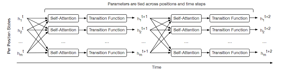
It can be seen that this recursive concept is very concise and easy to understand: the hidden state at time t undergoes complete computation of a single-layer Transformer module to obtain the hidden state at time t+1, which then undergoes this computation again to get the hidden state at time t+2, and so on in a cycle… To determine when this cycle ends, the article introduces Adaptive Computation Time (ACT): since different tokens have varying semantic ambiguity, some tokens naturally require more computation cycles. Therefore, ACT adds a halt flag for each token, which is computed normally within the model along with the entire sequence. When a token’s halt flag reaches the stop signal, that token’s hidden state is simply copied to the next time step until all sequences are marked as stopped, or the total number of cycles reaches the pre-set maximum.
It should be additionally noted that under this recursive strategy design, if the number of cycles is fixed at k, then this model is equivalent to a multi-layer Transformer model where all layer parameters are identical and tied. Moreover, the cycling dimension doesn’t iterate sequentially token by token from the first token like traditional RNNs, but rather iterates at the entire sequence computation level.
The experiments in this paper are also designed from the perspective of comparing Transformer and RNN models. For example, the bAbi QA dataset aims to measure various forms of language understanding ability by requiring specific types of reasoning on language facts presented in each story. The classic Transformer model performs poorly on this task (the authors note that they overfit under different hyperparameter settings), but if using Universal Transformer (UT) design, good results can be achieved. Meanwhile, classic RNN models can also handle this task, so the authors infer that UT combines the advantages of both Transformer and RNN models. On the Subject-Verb Agreement task, UT shows improvements over both Transformer and RNN model performances. On the LAMBADA task, RNN performs poorly, the Transformer model can handle it, and UT performs even better.
In summary, as one of the early articles introducing recursive concepts into Transformer model architectures, this article well demonstrates that recursive strategies can indeed improve model performance within Transformer models.
Lessons on Parameter Sharing across Layers in Transformers (SustaiNLP 2023)
Lessons on Parameter Sharing across Layers in Transformers
arxiv.org/abs/2104.06022
This article is also one of the earlier papers on recursive-related work and can be seen as an important bridge between the previous Universal Transformer and today’s Recursive LLMs. It points out the important limitations of UT’s recursive structure design, achieving similar iterative computation purposes through iterative computation between different layers in multi-layer Transformer models, while also reducing the number of effective model parameters.
Under the Universal Transformer model’s design structure, the entire Transformer model has only one layer, treated as a complete iterative block. Therefore, performing iterative computation k times on the original model requires k times the computational time, making this design impractical for larger model structures. Therefore, this article considers achieving similar iterative computation purposes through parameter sharing between different layers in multi-layer Transformer models, while also reducing the number of effective model parameters.
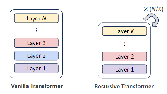
For example, as shown in the figure below, in a Transformer model with N=6 layers, designing the number of effective parameter groups as M=3, this creates a recursive structure where every N/M=2 layers share the same model parameters. Regarding the structured approach for which two layers share parameters, this article provides three schemes:
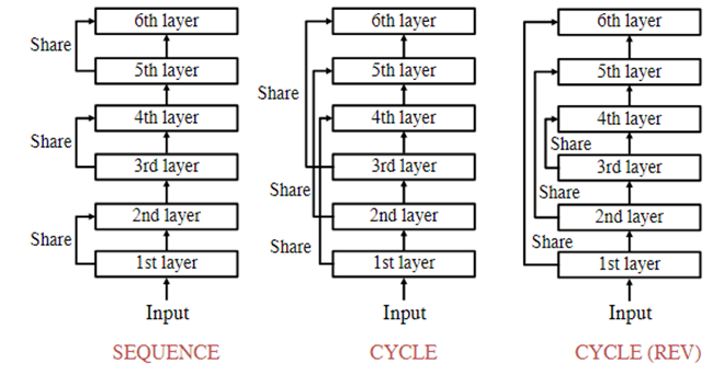
- Sequence mode: Execute in natural order, first completing the first shared parameter block (first computing the entire first Recursive block), then executing the second… until completion
- Cycle mode: Iterative computation occurs after all independent layers are computed, equivalent to computing layers 1, 2, 3 first, then going back to cycle compute again
- Cycle-Rev reverse cycle mode: Similar to Cycle mode, but the iterative computation order reverses to 3, 2, 1
Interestingly, the paper emphasizes that there is no obvious good or bad distinction among these three modes. In practice, which iterative computation scheme to adopt largely depends on the Transformer model’s own structural design, such as pre-norm and post-norm architectures. For example, for post-norm models, previous papers have found that earlier layers have larger gradient norms, especially during the warm-up phase. In other words, later layers have more parameter redundancy compared to earlier layers. Therefore, in this case, the Cycle-Rev reverse cycle mode can better utilize this portion of parameters. In the article’s experiments, they found that the Cycle mode performs slightly better.
This iterative computation design relaxes UT’s approach of directly performing recursive computation on an entire large Transformer layer, allowing equivalent effects to UT using fewer computational resources. The article conducted experiments on tasks like machine translation, showing that their method, when model parameters are the same (M = 6 and N = 12), has shorter computational time than UT while achieving slightly better BLEU scores than general strategies. On certain specific tasks, it even outperforms general Transformer models.
Relaxed Recursive Transformers: Effective Parameter Sharing with Layer-wise LoRA (ICLR 2025)
Relaxed Recursive Transformers: Effective Parameter Sharing with Layer-wise LoRA
arxiv.org/abs/2410.20672
After introducing the previous two background-oriented articles, we now come to the LLM domain. As is well known, LLMs generally follow the “big force creates miracles” approach, but this design places enormous computational resource demands. Through iterative computation design, computing certain parameters multiple times allows the actual computed parameters to remain unchanged while the actual parameters become fewer. This is a typical method of achieving parameter efficiency through Recursive computation.
This “Relaxed Recursive Transformers: Effective Parameter Sharing with Layer-wise LoRA” paper aims to implement this strategy. They target already pre-trained checkpoints (such as the Gemma 1B model) to initialize a smaller model, then perform finetuning with recursive computation on this small model, expecting to recover the same final performance as the original “full-size” model. To make the small model’s generalization ability stronger, they also add a layer-specific LoRA layer during each iteration, allowing the model to have potentially better performance while sharing weights.
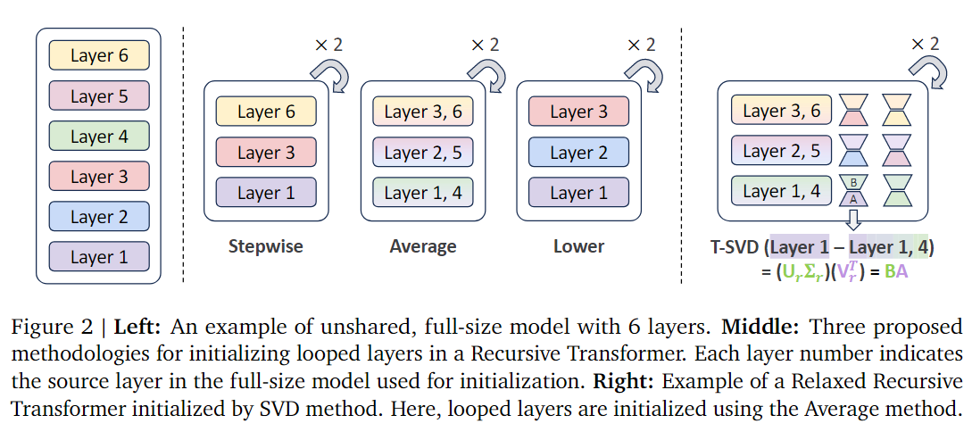
Their method of using already trained parameters to initialize small model parameters is called Looped Layer Tying. For example, they convert an 18-layer Gemma 2B model into a small model containing only 9 layers, making the overall iterative computation steps 2 times. Regarding how to “tie” these weights together, the paper proposes several methods, such as stepwise (selecting every other layer), average (mathematical averaging), lower (selecting only earlier layers). Through ablation experiments, they found that the Average approach achieves the best performance. The LoRA layer weight initialization uses the traditional singular value decomposition method for initialization. Figure 2 well visualizes these initialization strategies.
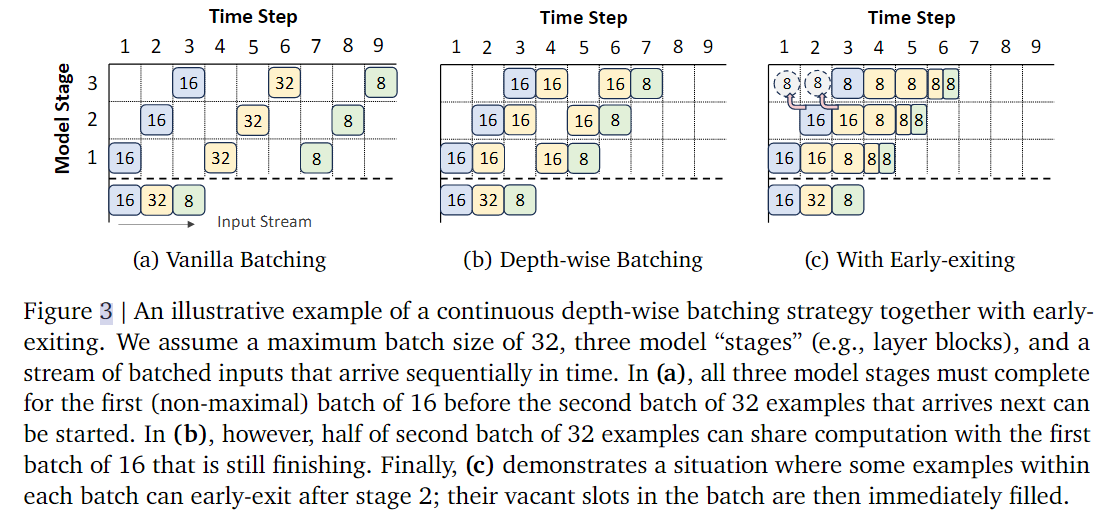
Additionally, at the system level and in practical deployment, user requests arrive asynchronously and continuously. Traditional Transformer inference must wait for all sequences in an entire batch to finish processing before accepting new requests, leading to low computational utilization. To solve this problem, past research proposed Continuous Sequence-wise Batching, where when a sequence generation completes, it’s immediately replaced with a new request to maintain maximum batch efficiency. This paper further proposes a new idea—Continuous Depth-wise Batching:
- Each layer in an ordinary Transformer is a different module, while Recursive Transformer shares the same function across all layers (recursive structure), so different samples can be computed simultaneously in different “depth cycles”.
- This way, the model can not only perform dynamic batching on the sequence dimension but also achieve dynamic parallelism on the “layer depth” dimension, thus maximizing GPU utilization.
- Additionally, this method combined with early-exiting can further accelerate. When some samples complete early, the freed computational positions can be immediately allocated to new requests. The recursive structure also naturally solves the common “waiting synchronization” problem in early-exit models (where some samples still need to wait for other samples after exiting). Figure 3 shows their system optimization strategy:
From the results in Figure 4, if the original model (pentagram) is directly shrunk without other operations, its few-shot accuracy evaluation results will decrease significantly (triangle). But after finetuning with recursive computation, the small model’s capability can recover much (circle), and with the relaxation strategy proposed in the paper, it can achieve performance close to or even better than the original model (rectangle). However, it’s worth noting that the introduction of LoRA parameters also increases model size. While more LoRA brings better results, there needs to be a balance between effectiveness and final effective model parameter count.
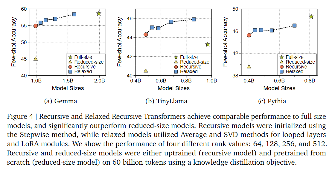
It’s worth noting that the paper’s ultimate goal is to have recursive Transformers achieve performance comparable to the original complete model without requiring extensive additional training. However, they found that distribution differences between pre-training datasets and additional training (uptraining) datasets can cause performance degradation. If new uptraining datasets have lower quality or different distributions, it can cause model degradation on certain benchmarks. For example, for the Gemma model, it was originally pre-trained using a high-quality, unpublished dataset, but when continued training on the lower-quality SlimPajama dataset, the model’s few-shot performance gradually declined, indicating that SlimPajama dataset’s “performance ceiling” itself is lower than the original data. Therefore, in Figure 5, the authors set different performance reference standards for different models. For Gemma and Pythia, they use “complete model performance with the same uptraining tokens” as the target; while for the TinyLlama model, since it was pre-trained on the SlimPajama dataset (same as the authors’ uptraining dataset, with no distribution bias), they directly use its original checkpoint performance as reference.
Additionally, the paper presents the performance of their proposed Continuous Depth-wise Batching in system-level throughput, and also conducts ablation experiments on other parameters mentioned in the paper, which won’t be elaborated here.
Mixture-of-Recursions: Learning Dynamic Recursive Depths for Adaptive Token-Level Computation (ICML 2025) ⭐
Mixture-of-Recursions: Learning Dynamic Recursive Depths for Adaptive Token-Level Computation
arxiv.org/abs/2507.10524
This article is personally considered one of the most suitable for close reading in the series of articles using recursive computation to increase parameter efficiency. This article synthesizes the ideas of parameter sharing and selective computation, applying the Mixture-of-Expert concept to recursive computation frameworks and naming it Mixture-of-Recursions.
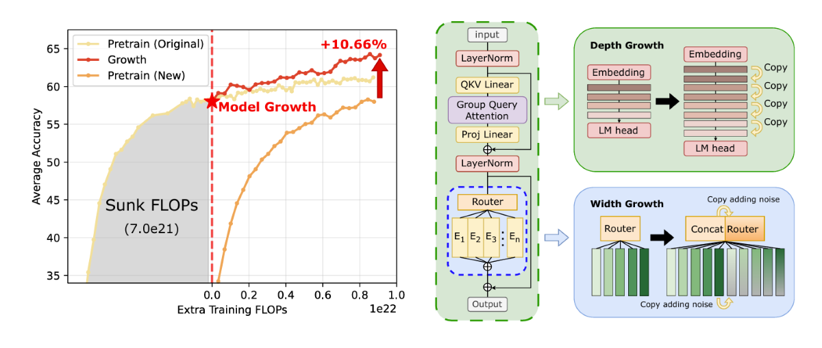
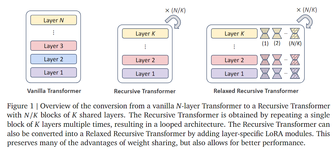
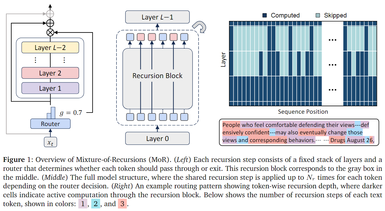
Traditional recursive networks have the entire input sequence perform recursive computation several times on the model, supplemented by some exit strategy to determine when to end the recursive computation. This article, while preserving the design of recursive computation for several layers in the Transformer layer, innovatively proposes to dynamically allocate different iterative computation counts for different tokens in the sequence. By adding a trainable lightweight Router at the front of the Transformer Block, it decides which important tokens need to be allocated for more computation, while those that are not very important can compute fewer times. As shown in Figure 1 below, the entire Mixture-of-Recursion model structure is relatively clear, and from the visualization, it can be seen that tokens with different semantic importance are allocated different numbers of recursive computation counts through this Router.
In the main text, the authors elaborate on the thought process behind this model design scheme. The entire MoR structure contains two key mechanisms:
- Routing mechanism: Decides how many recursive steps each token needs to go through;
- KV caching strategy: Decides how each recursive step reuses or selects attention cache (Key-Value pairs).
For the routing mechanism, the authors propose two routing strategies:
The first is called Expert-choice Routing. This idea directly comes from the top-k gating strategy in MoE models: each recursive depth is viewed as an expert, and each step selects the top-k tokens it wants to process. For the r-th recursive step, scores $g_r^t=G(\theta_r^T H_t^r)$ are calculated based on the current hidden state $H_t^r$ to obtain tokens with scores higher than the percentile threshold $P_{\beta}(G_r)$, which continue to recurse, otherwise they stay; and only tokens selected in the previous layer can enter the next layer (to conform to the logic of only computing the second time after computing the first time). This is equivalent to learning an “early-exit” mechanism during training, allowing higher layers to only process the most difficult tokens. This method can ensure computational load balance (each layer has a fixed number of tokens), but may generate information leakage—in that future information might be utilized when selecting tokens during training.
The second is called Token-choice Routing. Each token initially decides how many recursive steps it needs to go through. Scores $g_t$ for each “expert” (recursive depth) are calculated based on the initial hidden state $H_t^1$, the highest scoring one $i = \arg\max_j g_t^j$ is selected, and then this token is fixed to recurse $i$ times. Under this method, each token independently decides “how deep reasoning it needs,” rather than each layer deciding, avoiding causality destruction caused by future information. However, the disadvantage is that it’s easy to cause load imbalance (some tokens run multiple times, some only once), requiring additional load balancing losses or lossless algorithms to correct.
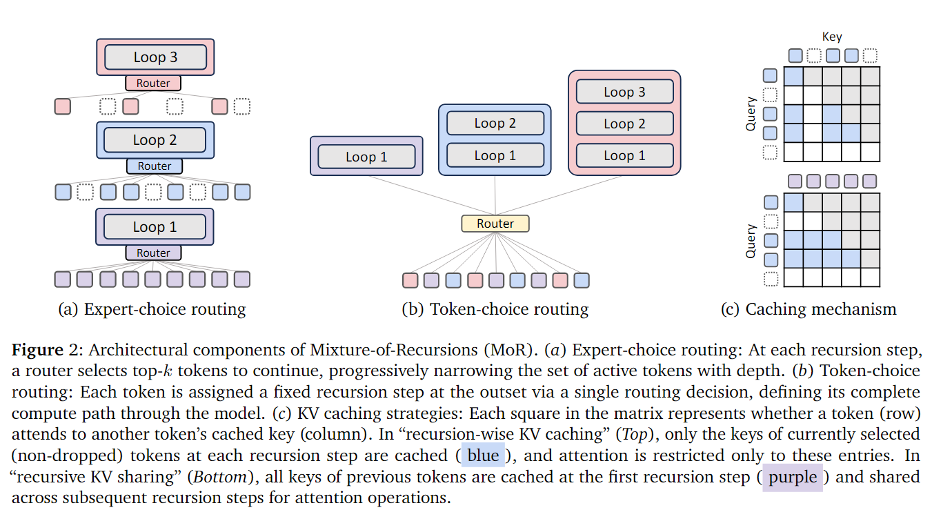
Figures (a) and (b) in the above Figure 2 vividly illustrate the differences between these two routing strategies. In Section 4.2, the authors analyze the impact of different design options in the MoR framework through a series of ablation experiments: For Expert-choice routing, discussing how to mitigate causality disruption (information leakage), the role of different normalization functions, router structures, and auxiliary losses; for Token-choice routing, discussing how to achieve load balance and routing stability. There’s no right or wrong issue with these two designs—different design schemes require different training details. The authors’ final experimental conclusion is that if using Expert-choice routing, auxiliary loss needs to be added, using Sigmoid normalization function, linear Router, z-loss is optional but has minimal impact on overall performance; if using Token-choice routing, load-balancing loss needs to be adopted, using Softmax activation function + MLP form Router, supplemented by slight z-loss.
Besides recursive mechanism design, the authors also propose a novel KV caching mechanism, referencing Figure 2(C). Traditional KV Cache strategies are not suitable for MoR structures because different tokens have different iterative computation counts, leading to KV missing and cache inconsistency issues caused by certain tokens exiting early. Therefore, the authors also propose two KV Cache strategies:
-
Recursion-wise KV Caching: Only caches the KV pairs of tokens routed to that layer in the current recursive layer, with each layer’s cache size precisely determined by capacity factors or load balance ratios. This strategy allows attention computation localization, significantly reducing memory usage and I/O pressure, with FLOPs costs decreasing proportionally (proportional to the square of token count), significantly improving efficiency.
-
Recursive KV Sharing: Only caches KV in the first recursive layer and reuses these caches in all subsequent recursive layers. This way, all tokens can always access complete context without repeated computation, significantly reducing memory and prefill phase overhead, but FLOPs reduction is limited and may be constrained by I/O bottlenecks.
Through ablation experiments and analysis, the authors found that in Recursive Transformers, KV sharing has almost no impact on performance. Despite parameters being shared across different depths, models remain relatively robust to KV sharing. Experiments found that KV representations at different recursive depths have similar magnitude distributions and high cosine similarity, so sharing KV only causes slight performance degradation. In the MoR (Mixture of Recursions) framework, different routing strategies perform differently: For Expert-choice routing, KV sharing significantly reduces performance; because such models need to focus only on active tokens at each layer, independent caching is more effective. For Token-choice routing, however, KV sharing is beneficial; due to its lower routing precision, shared KV additional context can help supplement information and improve overall stability.
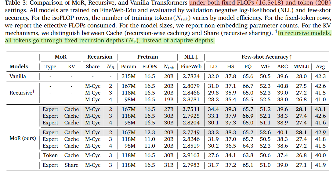
At the experimental level, the authors pre-trained models from scratch based on the Llama architecture (referencing SmolLM configuration) on the FineWeb-Edu dataset and evaluated performance on multiple few-shot benchmarks, comparing with normal Transformer, classical Recursive Transformer, and the proposed MoR. Main results are as follows (referencing Table 3):
-
Under the same computational budget (equivalent FLOPs), MoR is more efficient. MoR (2-layer recursion + expert-choice routing) achieves higher few-shot average accuracy under the same 16.5e18 FLOPs training budget than Vanilla (43.1% vs 42.3%); parameter count reduced by nearly 50%; due to higher computational utilization, more tokens can be processed under the same computation amount.
-
Under the same data volume (equivalent training tokens), MoR is more computationally efficient. Under fixed 20B token conditions: MoR (2-layer recursion) is superior to both Vanilla/Recursive; training FLOPs reduced by 25%, time shortened by 19%, peak memory reduced by 25%.
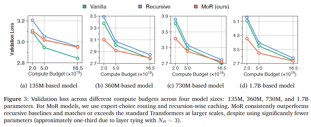
In addition, the paper conducted IsoFLOP (equivalent computation) analysis to verify whether MoR can still maintain or even improve performance when model scale and computational budget expand simultaneously? From Figure 3, the conclusion can be drawn that on small-scale models (135M), MoR is slightly below Vanilla, due to insufficient recursive capacity (i.e., shared weights limiting small model expressiveness). However, on medium-to-large-scale models (>360M), MoR performance quickly catches up and surpasses Vanilla, especially performing better under low/medium computational budgets. Therefore, MoR performs stably under the same computational budget with good scalability. Due to parameter sharing, MoR has higher parameter efficiency (i.e., fewer parameters achieving equivalent or better performance). Under the same FLOPs, MoR is a scalable, energy-efficient alternative architecture suitable for large-scale pre-training and deployment.
Hierarchical Reasoning Model & Less is More: Recursive Reasoning with Tiny Networks
Hierarchical Reasoning Model
arxiv.org/abs/2506.21734
Less is More: Recursive Reasoning with Tiny Networks
arxiv.org/abs/2510.04871
The final two articles are recently proposed models that have become very popular on the internet: HRM (Hierarchical Reasoning Model) and TRM (Tiny Recursive Model). They both claim to defeat DeepSeek-level large LLMs on certain reasoning tasks using extremely small networks. For example, the HRM model contains only 27M parameters and requires training from scratch on only 1,000 training data points to achieve results surpassing DeepSeek R1, Claude 3.7, and o3-mini-high on the ARC-AGI task. TRM is even more extreme, containing only 2 Transformer layers with just 7M parameters, achieving results on the ARC-AGI task that are even better than HRM, truly pushing parameter efficiency to the extreme.
However, careful analysis of these two articles reveals that although they achieve extreme parameter efficiency through iterative computation, both models are specialized neural networks designed for unique downstream tasks and completely cannot be considered within the LLM domain. Although they indeed solve the ARC-AGI task (similar to grid-filling, Sudoku-type problems) that current LLMs cannot handle well, we’ll only briefly focus on their insights regarding Recursive concepts without extensive elaboration.
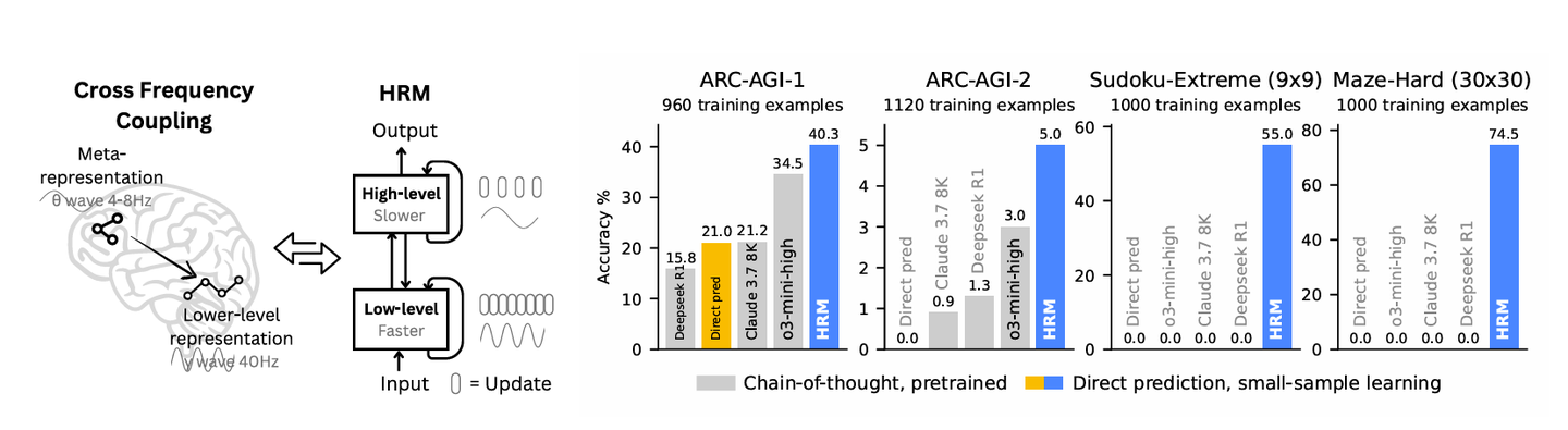
Let’s start with HRM (Hierarchical Reasoning Model). The article argues that existing LLM reasoning capabilities mainly rely on Chain-of-Thought prompting (CoT prompting), which decomposes tasks step by step at the language level. However, this approach has obvious problems, such as reasoning depending on “language expression,” performing poorly on graphic reasoning problems like ARC-AGI Sudoku tasks, requiring large amounts of data and generating long text, resulting in slow and inefficient reasoning. The authors propose that models should perform reasoning in hidden space, completing computation in internal hidden states rather than explicitly unfolding through language, as this approach is closer to the human brain: different cortical regions operate at different time scales. High-level regions perform slow, abstract reasoning while low-level regions perform fast, detailed processing.
Therefore, the authors referenced the hierarchical structure of the human brain to propose HRM: it has a dual-module structure where the high-level module (H) handles abstraction and slow reasoning, and the low-level module (L) handles fast, local computation. From a mathematical perspective, both actually share hidden states, but the H module’s update frequency is much slower than L. This can be understood as the L module experiencing T time-step cycles before conducting one H module computation. In this way, both alternate working, forming “hierarchical convergence”: after the L module updates multiple times to reach local stability, the H module then moves forward one step.
Additionally, the authors proposed a Deep Supervision design, essentially adapting training algorithms for this multiple iterative computation. Following traditional RNN-like training algorithms, models need to compute gradients and update parameters at each time step, making such loop structures difficult to train due to high computation and memory costs. This article proposed “one-step gradient approximation,” mathematically condensing the L module’s T-step iterative computation into a single gradient update, treating this approach in the algorithm as depth supervision signals propagated after several iterative computations. This approach reduces training memory complexity from O(T) to O(1), making training more efficient and more biologically feasible.
TRM is even more streamlined than HRM, removing the two-layer H-L reasoning structure and naturally integrating hidden states into the model computation process. Given input x, besides the first step where two-layer Transformers directly compute prediction result y from x, subsequent iterative computation processes will also use output z (hidden state) as input, utilizing x, the previous step’s y and z to update this step’s hidden state z, repeatedly iterating N times, allowing the model to continuously reflect on itself in hidden space. In addition, TRM also abandoned gradient approximation in deep supervision, switching to real complete gradient backpropagation. Finally, on the ARC-AGI task, HRM achieved 40% accuracy, while TRM achieved 45%.
Summary
It can be seen that Recursive Models have good effects in improving parameter efficiency, and with the current trend of increasingly large LLM parameters, their application scenarios are becoming more extensive. Moreover, from another perspective, when computational resources are relatively abundant, we can increase model reasoning capabilities by simply increasing the number of iterative computation steps without changing model parameter count, a direction mentioned more or less in the above articles on parameter efficiency. I will next write another article to continue summarizing research articles specifically focused on Recursive model performance in reasoning tasks.