5,000 words Analysis of FP4 Quantization for Training Large Language Models
Published:
This blog is also available in Chinese version: https://zhuanlan.zhihu.com/p/1910768186401466238
Detailed Paper Interpretation of “Optimizing Large Language Model Training Using FP4 Quantization”
Low-bit data formats are no stranger to most of us. Compared to the default floating-point format used in computers (FP32), lower-bit formats in AI—especially in large language model (LLM) training and inference—not only reduce memory consumption but can also accelerate computation when paired with specialized hardware. Moreover, with proper optimization algorithms or frameworks, these formats can maintain model accuracy.
Today, I’d like to share a gentle yet insightful discussion on the application of low-bit data formats in LLM training. We specifically explored the use of FP4 format in LLM training, identified key challenges, and have compiled our findings into a paper:
📝 Optimizing Large Language Model Training Using FP4 Quantization
arXiv:2501.17116
Unlike typical “hardcore” paper analyses, this post aims to walk you through the motivation, key insights, and design rationale behind our work—why we did it, how our methods were conceived, why we chose them, and how we arrived at our results.
Quick Links:
- 📝 Paper: Optimizing Large Language Model Training Using FP4 Quantization
- 💻 GitHub: https://github.com/Azure/MS-AMP
Background and Motivation
By default, computers represent a floating-point number using four bytes (32 bits), known as FP32. In deep learning, we also commonly use BF16/FP16 (2 bytes), FP8 (1 byte), and even formats as low as 4 bits (half a byte) or 1 bit. NVIDIA’s H-series GPUs offer native support for FP8, enabling 2× higher throughput for matrix multiplication compared to FP16. Even more impressively, upcoming B-series GPUs are expected to support FP4, potentially doubling FP8 throughput again.
This suggests tremendous potential for reducing training costs if such ultra-low-bit formats can be applied to LLM training.
However, as the saying goes: there’s no free lunch. While low-bit formats offer speed advantages, they suffer from severely limited precision. Fewer bits mean a narrower dynamic range, risking overflow (values too large) or underflow (values too small), and larger quantization (rounding) errors due to coarser representable intervals. For example, 1-bit can only represent ±1; 4-bit yields just 16 distinct values.
As shown in Figure 1, when we directly quantize a LLaMA2-400M model to FP4 during training, the model suffers catastrophic precision loss and fails to converge.
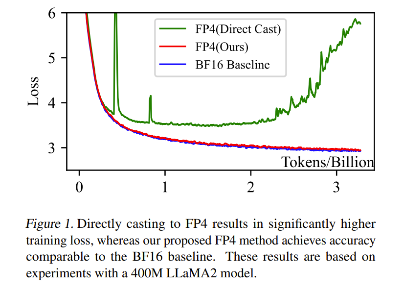
Figure 1: Training loss curves.
- Blue: BF16 baseline (converges normally).
- Green: Naive FP4 quantization (diverges).
- Red: Our proposed FP4 training framework (converges well).
Thus, to harness the power of ultra-low-bit computation in LLM training, we must carefully design methods to preserve model accuracy.
What Is FP4?
You might wonder: “With only 4 bits, there are just 16 possible values—how can that possibly train a large model?”
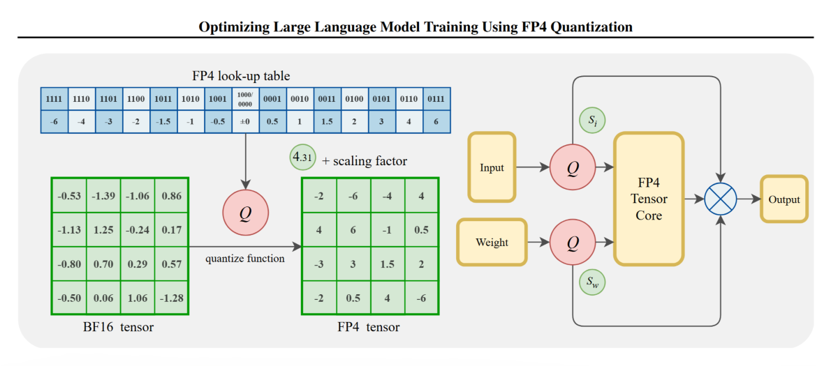
This is actually still a fairly critical issue. When we talk about data quantization in large language models, it certainly doesn’t mean simply using the numbers 1/2/3/4…15/16 to train these large models. Currently, quantization applied during training or inference of large models is typically “scaled quantization.” Specifically, the original tensor (which follows a certain data distribution) is scaled based on its maximum absolute value and the maximum absolute value representable by a low-bit format such as FP4 (or other low-bit formats). A scaling factor is computed from these two values, and the original tensor is scaled by this factor before being quantized. This approach is known as “max-abs quantization” (quantization based on the maximum absolute value). If, instead of the maximum absolute value, the mean value is used, it is called “mean-based quantization.”
Max-abs quantization can be expressed mathematically as follows:
\[x_{\text{fp4}} = \textit{Q}(x_{\text{fp16}} \cdot \gamma), \quad \gamma = \frac{\text{MAX}_{\text{fp4}}}{\text{max}(|x_{\text{fp16}}|)}\]The effect of the scaling factor on quantization can be intuitively understood from the figure below. Recall that a floating-point number is represented as:
\[\text{Value} = (-1)^S \times (1.M) \times 2^{E - \text{bias}}\]Multiplying the value by a scaling factor is mathematically equivalent to adding or subtracting from the exponent field E . If we use a log₂ scale, this operation can be viewed as a shift along the exponent axis. As illustrated in the figure, the original blue tensor exceeds the representable range of the FP8 format, causing all tensor values below the red line to become zero after quantization. After applying the scaling factor, the entire original tensor is shifted leftward (in the log₂ coordinate system) into the green region, thereby bringing it within the representable range of the FP8 format.
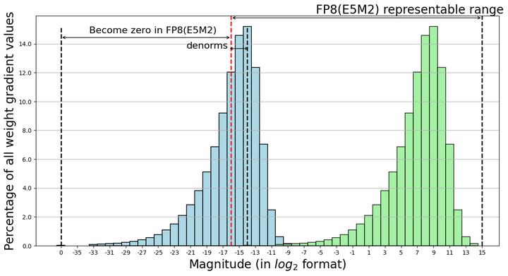 Figure 2: Visualization of scaling effect in low-bit quantization using log₂ scale. The scaling factor shifts the entire tensor into the representable range.
As illustrated:
- The original blue tensor exceeds the representable range of the FP8 format
- All tensor values below the red line become zero after quantization
- After applying the scaling factor, the entire original tensor is shifted leftward (in the log₂ coordinate system) into the green region, bringing it within the representable range However, the way we determine the group of tensors to which this scaling is applied differs from that used for FP8. This distinction relates to the granularity of quantization—a rather nuanced and complex topic—which we won’t delve into further here.
According to the IEEE standard, when all bits of the exponent field (E) are set to 1, the resulting bit pattern does not correspond to a valid finite number. Specifically, if the mantissa (M) is all zeros in this case, it represents infinity (Inf); if the mantissa contains any non-zero bits, it represents a NaN (Not a Number). However, due to the extremely limited bit width of FP8 and FP4 formats, this IEEE rule is typically ignored, as the primary goal becomes maximizing the representation of meaningful numerical values. For instance, the FP8 (E4M3) format does not define Inf, and FP6 and FP4 formats omit both Inf and NaN entirely.
For a detailed numerical specification of FP4, please refer to the accompanying table and figure. Since FP4 can represent only 16 distinct finite values, we have enumerated all of them explicitly. As shown, one bit in FP4 is already reserved for the sign. Among the remaining three bits, allocating more bits to the exponent (E) increases the dynamic range, while allocating more bits to the mantissa (M) yields finer quantization granularity. To strike a practical balance between dynamic range and precision, we adopt the E2M1 format for FP4.
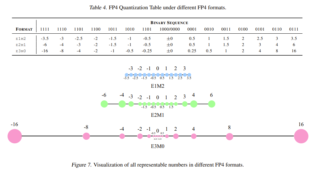 Figure 3: FP4 format specifications. E2M1 provides optimal balance between range and precision, with all 16 representable values explicitly shown.
Methodology
In practical training, to fully leverage the computational efficiency of Tensor Cores, both input tensors of a matrix multiplication must be quantized to a low-precision format before performing the forward matrix multiplication:
- 📦 Weight tensor
W - 💡 Activation tensor
A
However, as previously discussed, directly quantizing these tensors to FP4 would lead to severe accuracy degradation. To address this, we have developed two distinct strategies:
- 🎯 Differentiable Gradient Estimator (DGE) → preserving weight precision
- ✂️ Outlier Clamping and Compensation (OCC) → maintaining activation fidelity
1. Differentiable Gradient Estimator (DGE)
During training, backpropagation requires computing gradients through quantized weights. But quantization is non-differentiable—it’s a step function with discontinuities, making gradients undefined at quantization boundaries.
During neural network training, every operator must support not only forward propagation but also backward propagation to compute gradients for parameter updates. Backpropagation is essentially a differentiation process: using the chain rule, gradients are propagated backward from the final layer all the way to the first, enabling gradient computation for each layer.
However, as is well known, the quantization function is non-differentiable. Its graph exhibits discontinuous jumps at quantization boundaries—points where the left-hand and right-hand limits differ—making the derivative undefined at those locations. Consider a step function: at the step point, the theoretical gradient is infinite, and its derivative is a Dirac delta function. If we naively insert a quantization function into the training pipeline, gradient backpropagation would halt at this non-differentiable operation, which clearly contradicts our goal of end-to-end trainable quantization.
To circumvent this issue, a widely adopted approach is the Straight-Through Estimator (STE). Conceptually, STE assumes that the gradient of the quantized weights is equal to the gradient of the unquantized (full-precision) weights—an assumption we will justify with a simple theoretical argument shortly. In practice, STE implements this by simply bypassing the gradient of the quantization function during backpropagation: while the forward pass includes the quantization operation as usual, the backward pass ignores the (non-existent) derivative of the quantizer and directly passes the incoming gradient through unchanged. In other words, gradients flow backward exactly as they would in a network without quantization.
This method is extremely convenient and easy to implement in code. Yet it naturally raises a critical question: Is this gradient approximation truly accurate? Could it introduce hidden errors that impair training stability or final model performance?
To address this intuitive concern, we can briefly analyze how quantized weights are actually updated during training—i.e., how gradients propagate through the quantization operation. The forward pass can be expressed as:
\[Y = AW_q = Af(W)\]Where $ f $ is the quantization function.
During backpropagation, we compute the partial derivatives of the loss $ L $ with respect to the weights $ W $ and activations $ A $. Here, we focus only on the weights $ W $. Using standard matrix calculus and the chain rule, we obtain:
\[\frac{\partial L}{\partial W} = \frac{\partial L}{\partial W_q} \cdot \frac{\partial W_q}{\partial W} = \left( A^\top \frac{\partial L}{\partial Y} \right) \cdot \frac{\partial W_q}{\partial W}\]where $ \frac{\partial W_q}{\partial W} $ is the derivative of the quantization function. Note that the quantization function operates on a matrix input; theoretically, its derivative should follow matrix calculus rules. Fortunately, quantization is an element-wise function, so its derivative is also element-wise. Consequently, the term $ \frac{\partial W_q}{\partial W} $ in the above expression corresponds to a diagonal Jacobian matrix, and the matrix multiplication simplifies to an element-wise (Hadamard) product between $ A^\top \frac{\partial L}{\partial Y} $ and the element-wise derivative of the quantization function applied to each entry of $ W $.
For a more detailed derivation, please refer to Section 3.1 and the Appendix of the paper!
Here is the final key result:
\[\frac{\partial L}{\partial W} = \frac{\partial L}{\partial W_q} \odot f'(W)\]where:
- $ \frac{\partial L}{\partial W} $ is the gradient of the loss with respect to the original (full-precision) weights—commonly referred to as the weight gradient.
- In optimizers like Adam, the weight update rule is $ W_t = W_{t-1} - \eta \cdot \Delta W_{t-1} $, where $ \Delta W_{t-1} $ is essentially $ \frac{\partial L}{\partial W} $ (ignoring first- and second-moment momentum terms for simplicity).
- However, in actual training, what we directly compute is $ \frac{\partial L}{\partial W_q} $—the gradient of the loss with respect to the quantized weights—because during the forward pass, $ W $ has already been quantized to $ W_q $, and backpropagation naturally starts from $ W_q $.
From the formula above, we see that the desired weight gradient $ \frac{\partial L}{\partial W} $ differs from the actually computed gradient $ \frac{\partial L}{\partial W_q} $ by a factor of $ f’(W) $—the derivative of the quantization function with respect to the original weights $ W $. Multiplying $ \frac{\partial L}{\partial W_q} $ element-wise by $ f’(W) $ yields the true gradient $ \frac{\partial L}{\partial W} $ that we want.
However, the quantization function $ f $ is non-differentiable, so under normal circumstances, $ f’(W) $ cannot be computed. In the Straight-Through Estimator (STE) approach, we simply assume that $ f’(W) \equiv 1 $ (i.e., the derivative is identically 1), thereby bypassing the need to compute this derivative altogether. This is precisely why, theoretically, STE assumes that the gradient with respect to the quantized weights is equal to the gradient with respect to the original (unquantized) weights.
The main advantage of this assumption is its simplicity in implementation. In practice, to implement an STE-based custom autograd function in PyTorch, one only needs to apply quantization in the forward method and, in the backward method, directly pass the incoming gradient through as the outgoing gradient (i.e., set input and output gradients equal).
This assumption also has some theoretical justification: if $ f’(W) = 1 $, it implies that the forward function behaves like $ f(W) = W $—in other words, the quantization is so accurate that the quantized weights are nearly identical to the original weights, with negligible quantization loss.
However, in ultra-low-bit quantization scenarios (e.g., FP4), this assumption inevitably introduces error—because we know that the quantized tensor is always different from the original tensor, and the lower the bit-width, the larger this discrepancy (i.e., the greater the quantization error).
Therefore, we ask: Can we mitigate this error? Returning to the core formula, if we could compute a more accurate approximation of $ f’(W) $, the resulting weight gradient would naturally be more precise. Unfortunately, since the true quantization function is discontinuous and non-differentiable, we adopt a practical compromise: we approximate it with a steep but smooth, differentiable function. We then compute the derivative of this surrogate function and use it as a proxy for $ f’(W) $. This allows us to obtain a more accurate estimate of the true gradient.
In essence, $ f’(W) $ acts as a calibration term for the weight gradients, enabling more precise weight updates during training!
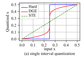 Figure 4: Comparison of quantization functions and their derivatives
Legend:
- 🔵 Blue line: Original non-differentiable quantization function (Hard)
- 🔴 Red line: Our DGE approach – approximating quantization using a steep yet differentiable function
- ⚫ Black dashed line: STE assumption (y=x) for comparison
With this insight in place, the next steps become clear. We select a shifted and scaled power function to approximate the quantization function and use its derivative as the crucial gradient calibration term $ f’(W) $. The function we adopt is defined as:
\[f(x) = \frac{\delta}{2} \cdot \left( 1 + \operatorname{sign}\left( \frac{2x}{\delta} - 1 \right) \cdot \left| \frac{2x}{\delta} - 1 \right|^{\frac{1}{k}} \right)\]The red curve in the figure above illustrates this function, where $ \delta $ denotes the quantization step size, and the hyperparameter $ k $ controls the steepness of the function. A larger $ k $ makes the function steeper, thereby better approximating the original (non-differentiable) quantization function.
The derivative of this function is:
\[f'(x) = \frac{1}{k} \cdot \left| \frac{2x}{\delta} - 1 \right|^{\frac{1}{k} - 1}\]In practice, during the forward pass, we directly quantize the weights $ W $. During backpropagation, we compute the calibration term $ f’(W) $ using the derivative formula above and apply it element-wise to the weight gradients to obtain more accurate weight updates.
For a detailed derivation of these two formulas and further technical nuances, please refer to Section 3.1 and Appendix C of the original paper—here we omit the full derivation for brevity.
We conducted ablation studies on the 1.3B LLaMA-2 model to validate the effectiveness of the Differentiable Gradient Estimator (DGE). In the notation W4A8, weights W are quantized to 4 bits while activations A remain at 8 bits—effectively a weight-only quantization setting. As shown in the convergence curves, incorporating the DGE correction term significantly improves training convergence compared to the gray-blue baseline (without DGE).
Regarding the hyperparameter k: larger values better approximate the true quantization function but can lead to instability in the gradient correction term. Empirically, a moderate value of k = 5 yields the best final performance, as illustrated by the green curve.
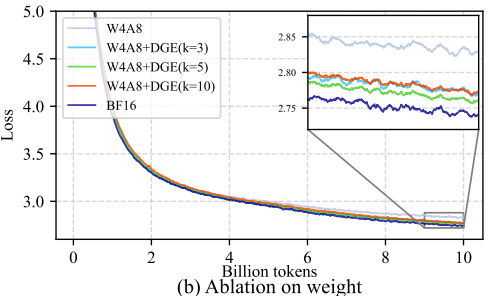 Figure 5: DGE ablation study on LLaMA-1.3B. The green curve (k=5) shows optimal convergence.
2. Outlier Clamping and Compensation (OCC)
Next, we turn to the quantization strategy for activation values A.
The Outlier Problem
During training or inference of large language models (LLMs), activation values—i.e., intermediate outputs from operators such as attention or MLP layers—are significantly harder to quantize than model weights. A key reason for this difficulty is the prevalence of outliers in activations.
To clarify, consider an activation tensor of shape, for example, 1024 × 4096. If we treat all its elements as samples from a distribution, outliers refer to those values whose magnitudes are substantially larger than the typical (e.g., mean or median) values in that distribution.
📈 For a detailed comparison between the statistical distributions of weights and activations, please refer to Appendix D of the original paper.
Numerous quantization studies have systematically investigated the characteristics of outliers in LLM activations. Key findings:
- ⚠️ Outliers are extremely common in LLM activations
- 🔄 They appear consistently across virtually all large language models during both training and inference
- 📉 These outliers tend to concentrate along specific channel dimensions (feature/hidden dimensions)
- ❌ Rather than along the orthogonal token dimension (sequence/batch dimension)
- 🎯 This phenomenon is known as channel-wise outlier distribution
Our experiments confirm this observation, as illustrated in the figure below:
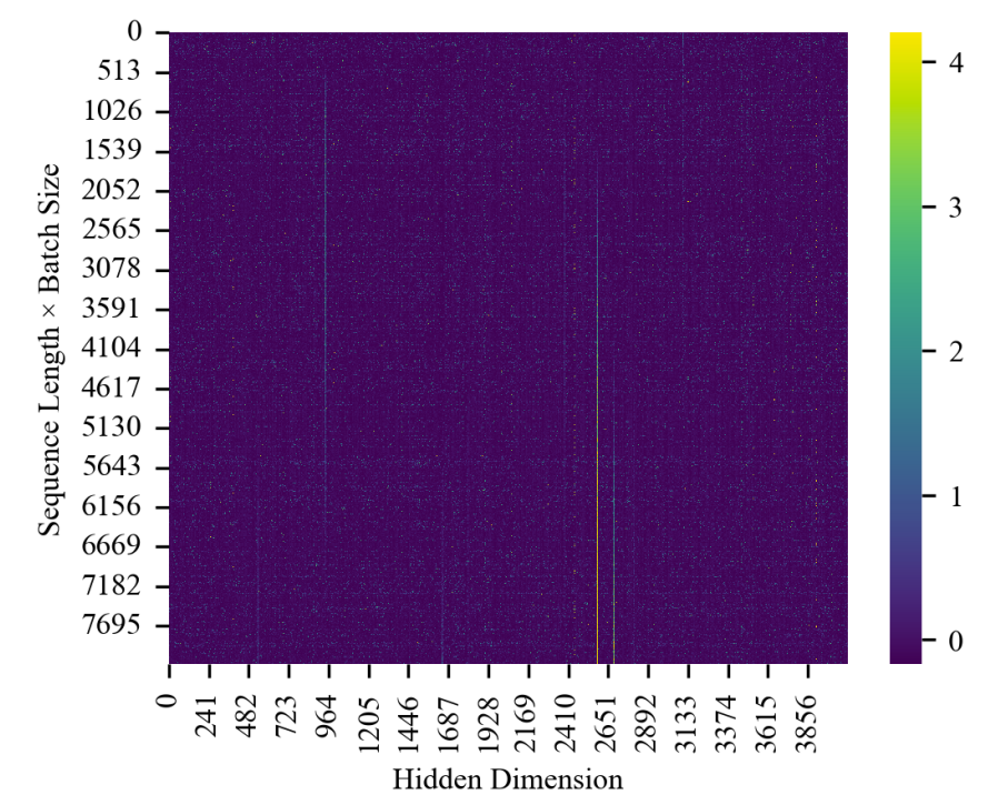 Figure 6: Heatmap of GeLU output activations from LLaMA-1.3B (iteration 30k). Light regions show outliers concentrated along specific hidden dimensions, demonstrating clear channel-wise pattern.
Observation: All extremely large values (light-colored regions) are concentrated along certain specific hidden dimensions—demonstrating a clear channel-wise pattern—while their distribution across the sequence × batch dimensions appears relatively uniform.
Unfortunately, the presence of such outliers is catastrophic for quantization. As previously described, in max-abs quantization, the scaling factor is computed based on the maximum absolute value in the original tensor and the largest representable value in the target format (e.g., FP4). When outliers are present, this maximum value is dominated by a few extreme entries that do not reflect the magnitude of the vast majority of values in the tensor. Consequently, the computed scaling factor becomes excessively large, causing most of the non-outlier values to be scaled down so much that they collapse to zero after quantization—rendering them effectively unrepresentable.
Based on this observation—and given our use of max-abs quantization—we propose an outlier clamping strategy. Specifically, we clamp the activation tensor to a pre-defined percentile (e.g., the 99th percentile), effectively capping values with excessively large magnitudes.
As shown in the figure below:
- Without clamping, the quantization function is heavily skewed by outliers in the original tensor. After FP4 quantization, the resulting values completely lose the original distribution, with a large portion of entries quantized to zero—introducing severe quantization error.
- With clamping, although the information from the top 1% extreme outliers is lost, the vast majority (~99%) of the tensor’s distribution is preserved. This leads to a much more faithful representation in low-bit quantization and significantly reduces overall quantization error.
Thus, outlier clamping strikes a practical trade-off: sacrificing a tiny fraction of extreme values to preserve the fidelity of the dominant signal in the activation tensor.
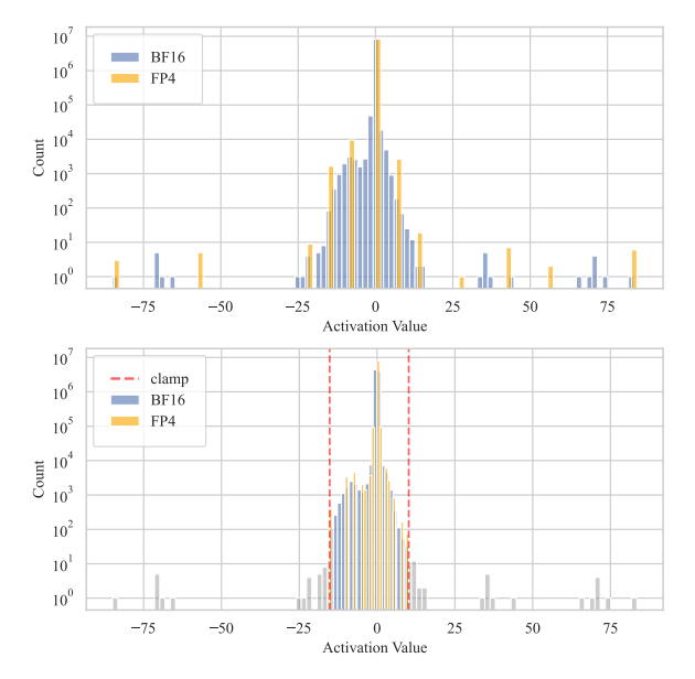 Figure 7: Comparison of quantization results with and without outlier clamping
Analysis:
- ❌ Top (Without clamping): The quantization function is heavily skewed by outliers. After FP4 quantization, the resulting values completely lose the original distribution, with a large portion quantized to zero—introducing severe quantization error.
- ✅ Bottom (With clamping): Although the information from the top 1% extreme outliers is lost, the vast majority (~99%) of the tensor’s distribution is preserved, leading to much more faithful representation and significantly reduced quantization error.
🎯 Trade-off: Sacrificing a tiny fraction of extreme values to preserve the fidelity of the dominant signal.
In addition to outlier clamping, we observe that the clipped outliers themselves still exert a non-negligible impact on final quantization accuracy. To further mitigate quantization error, we propose a high-precision compensation strategy to account for the influence of these removed outliers. The detailed procedure is illustrated in the figure below.
Because we use a high percentile threshold (e.g., 99th), clamping affects only a very small fraction of extreme values. In other words, if we decompose the original activation tensor as $Y = Y_c + \Delta Y$, where $Y_c$ represents the main body of the tensor (which will be quantized to low precision, e.g., FP4) and $\Delta Y$ contains the outliers, then $\Delta Y$ is highly sparse. This sparsity allows us to compensate for the missing information with minimal computational overhead: although the compensation uses higher precision (e.g., FP8), the associated matrix multiplication can be accelerated using sparse matrix multiplication techniques.
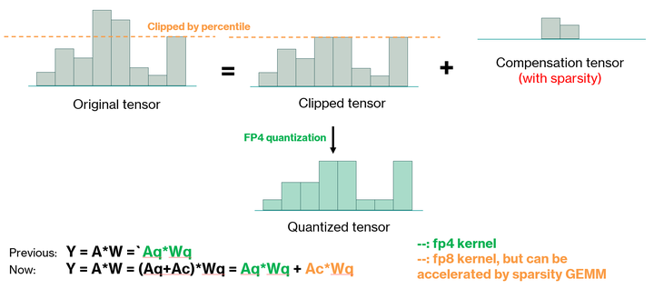 Figure 8: Outlier clamping and compensation strategy. The sparse compensation matrix ΔY enables high-precision correction with minimal overhead.
Key insight: Because we use a high percentile threshold (e.g., 99th), clamping affects only a very small fraction of extreme values. If we decompose the original activation tensor as Y = Y_c + ΔY:
Y_c= main body (quantized to low precision, e.g., FP4)ΔY= outliers (highly sparse)
This sparsity allows us to compensate for missing information with minimal computational overhead: although compensation uses higher precision (e.g., FP8), the associated matrix multiplication can be accelerated using sparse matrix multiplication techniques.
We also provide a quantitative analysis of this approach. The evaluation metrics are averaged over all activation matrices from the 1.3B LLaMA model at training iteration 30,000.
Quantitative Results:
| Clamp? | Comp? | Quantile | Cosine Sim ↑ | MSE ↓ | SNR ↑ |
|---|---|---|---|---|---|
| ✗ | — | — | 92.19% | 0.1055 | 8.31 |
| ✓ | ✗ | 99.9 | 98.83% | 0.0366 | 14.25 |
| ✓ | ✓ | 99.9 | 99.61% | 0.0245 | 15.31 |
| ✓ | ✓ | 99 | 100% | 0.0099 | 18.38 |
| ✓ | ✓ | 97 | 100% | 0.0068 | 20.88 |
Key findings:
- ✅ Outlier clamping significantly improves cosine similarity and signal-to-noise ratio (SNR)
- ✅ Reduces mean squared error (MSE) between original and quantized tensors
- ✅ Introducing compensation mechanism further reduces quantization error
⚖️ Trade-off: Lowering the clamping percentile (e.g., from 99% to 95%) reduces sparsity of the compensation matrix—expanding the set of outliers—thereby further decreasing quantization error. However, this comes at the cost of increased computational overhead for compensation.
We conducted ablation studies on the 1.3B LLaMA-2 model to validate the effectiveness of our Outlier Clamping and Compensation (OCC) scheme. In the notation W8A4, weights W are quantized to 8 bits while activations A are quantized to 4 bits—effectively an activation-only quantization setting.
 Figure 9: OCC ablation study showing stable convergence with different α values
Key observations:
- ❌ Without OCC: Directly quantizing activations to FP4 leads to training divergence—after a certain number of training steps, the loss spikes and becomes NaN
- ✅ With OCC: Outlier clamping together with compensation effectively closes this loss gap and ensures stable convergence
Hyperparameter α (clamping percentile):
- Smaller α → stronger compensation effect (more outliers treated) → higher accuracy but higher computational cost
- α = 0.999 → ~0.2% non-zero elements (light blue curve)
- α = 0.99 → ~2% non-zero elements (green curve)
- α = 0.97 → ~6% non-zero elements (orange curve)
🎯 Optimal trade-off: Considering both accuracy and speed, α = 0.99 offers the best practical balance.
Experimental Results
Our experiments are all conducted on the LLaMA model architecture, focusing on three model scales: 1.3B, 7B, and 13B. All these models are randomly initialized and trained from scratch. The training dataset used is the open-source DCLM dataset, and the tokenizer is the open-source LLaMA tokenizer.
In the forward pass of training, the matrix multiplication is expressed as $ Y = A \cdot W $, where
- $ A $ (of shape sequence length × input channels) is the activation tensor,
- $ W $ (of shape input channels × output channels) is the weight tensor.
To maintain consistency with the logic of matrix multiplication, we apply vector-wise quantization schemes in different directions for $ A $ and $ W $:
- The activation tensor $ A $ is quantized token-wise along the sequence length dimension,
- The weight tensor $ W $ is quantized channel-wise along the output channel dimension.
At the time of our experiments, FP4 Tensor Cores were not yet available, so we used NVIDIA H-series GPUs’ FP8 Tensor Cores to simulate FP4 computation. This is justified because the FP8 format fully covers the dynamic range of FP4.
In neural network quantized training, mixed-precision training has always been an unavoidable topic. In LLM training, general matrix multiplication (GeMM) accounts for over 95% of the total computational load, and this proportion further increases as model size grows. Therefore, we focus on quantizing GeMM operations to FP4, which aligns with the core capability envisioned for FP4 Tensor Cores.
Specifically, in our mixed-precision setup:
- Gradient communication in data parallelism uses the FP8 format,
- During optimizer updates, gradients and first-order momentum are stored in FP8,
- Second-order momentum is stored in BF16,
- Other operators (e.g., layer normalization, softmax, etc.) use higher-precision formats such as BF16 or FP32.
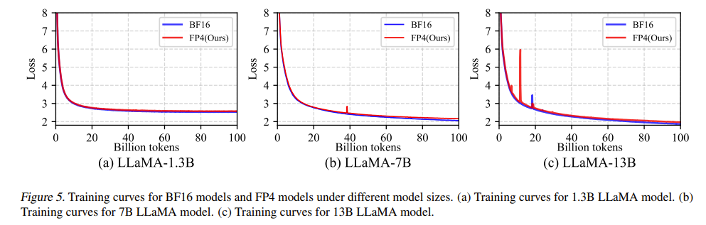
Convergence curves for 1.3B/7B/13B models; FP4 nearly overlaps BF16 baseline.
Figure 5 shows the convergence curves of models at the three scales. It can be seen that the FP4 curve and the BF16 baseline curve are almost overlapping. Specifically, after training on 100 billion tokens, the training losses are as follows:
- 1.3B model: 2.55 (FP4) vs. 2.49 (BF16),
- 7B model: 2.17 (FP4) vs. 2.07 (BF16),
- 13B model: 1.97 (FP4) vs. 1.88 (BF16).
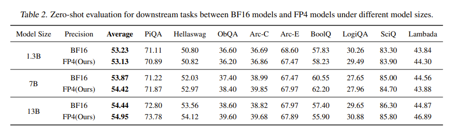
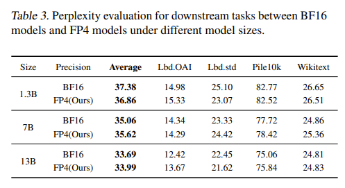
Downstream zero-shot QA accuracy (higher = better) and perplexity (lower = better), evaluated via lm-evaluation-harness.
Tables 2 and 3 present evaluation results of the three trained models on downstream task datasets, including zero-shot question-answering (QA) tasks and perplexity (ppl) metrics. Higher QA accuracy indicates better model performance; lower perplexity indicates better performance. All results are obtained using the widely adopted evaluation benchmark lm-evaluation-harness (GitHub: github.com/EleutherAI/lm-evaluation-harness).
From both vertical (across models) and horizontal (across precisions) comparisons in the tables, we observe that models trained in FP4 precision achieve performance nearly identical to those trained in BF16 precision, and all results follow the general trend that larger models yield better performance. For more training result details, please refer to the original paper.
In addition to the main experimental results, we also conducted a series of ablation studies. The ablation experiments for the DGE method (for weights $W$) and the OCC method (for activations $A$) have already been analyzed in earlier sections. We also performed other ablation studies.
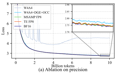
Ablation on computation precision
The figure shows an ablation study on computational precision, comparing:
- BF16 (baseline),
- MS-AMP FP8,
- Transformer Engine FP8,
- Direct FP4 quantization (denoted as W4A4, meaning both weights and activations are quantized to FP4),
- Our full FP4 method (W4A4 + DGE + OCC).
The results show that both FP8 methods and our FP4 method maintain training accuracy comparable to the baseline, whereas direct FP4 quantization exhibits a significant training loss gap. In the zoomed-in curve, it is visible that the loss of our FP4 method is still slightly higher than that of FP8 and BF16 methods.
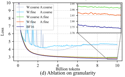
Ablation on quantization granularity caption
In our experiments, we also observed that quantization granularity is critical in FP4 quantization. Although FP8 training can achieve sufficient accuracy using coarse tensor-wise quantization, the figure shows that applying tensor-wise quantization in FP4 leads to significantly higher training error. To address this, we adopt vector-wise quantization: activations are quantized token-wise, and weights are quantized channel-wise—exactly as dictated by the GeMM computation rules discussed earlier.
Notably, applying coarse-grained quantization only to activations causes a more severe accuracy drop than applying it only to weights, indicating that activations are harder to quantize than weights—which directly aligns with our earlier discussion about the presence of outliers in activation values.
Summary
The application of low-precision formats in neural network training remains an extremely challenging topic. In the paper “Optimizing Large Language Model Training Using FP4 Quantization”, we propose applying the FP4 format to the neural network training process and successfully overcome the severe precision limitations inherent to the FP4 data format.
- To enable more accurate weight updates, we propose the Differentiable Gradient Estimator (DGE) method.
- To address the outlier problem in activation values, we propose the Outlier Clamping and Compensation (OCC) method.
From both training loss curves and downstream task evaluations, models trained using the FP4 format achieve results comparable to those trained using BF16.
Our research demonstrates the feasibility of training large language models using FP4 low-precision formats, provides valuable insights for improving ultra-low-precision quantization methods, and may also inspire the design of next-generation low-precision computing hardware to realize efficient 4-bit compute kernels.
Unfortunately, since we do not yet have access to dedicated FP4 Tensor Cores, we cannot directly measure the speedup achievable with native FP4 support. All experiments described above rely on FP4 simulation: for example, a BF16 tensor must first be converted to FP4 to simulate quantization, then converted again to FP8 to be fed into the Tensor Core for computation. This introduces additional precision conversion overhead, significantly reducing actual runtime speed.
Moreover, due to computational resource limitations, we have not yet extended our experiments to extremely large models (e.g., 100B or hundreds of billions of parameters) or extremely large datasets containing trillions (T-level) of tokens. Exploring the scalability of low-precision training remains a key direction for future research.
For more details and supplementary content, please refer to the main paper. We also welcome questions and discussion!
Optimizing Large Language Model Training Using FP4 Quantization
Paper link: arxiv.org/abs/2501.17116
Code Link: https://github.com/Azure/MS-AMP