This blog is also available in Chinese version: https://zhuanlan.zhihu.com/p/1934724931519743930

Quantization Scaling Laws: A Comprehensive Overview

Quantization has always been an effective means of saving costs in both large model training and inference. However, at the same time, overly low-precision formats can lead to degraded model performance. This naturally makes us wonder: is there a guiding principle that allows us to use the most appropriate data format in scenarios where we want to apply large model quantization (such as models of specified sizes)?

Fortunately, Quantization Scaling Law points us in the right direction. While ordinary Scaling Law reveals how the training loss of large language models changes with model parameter scale and total training token count, Quantization Scaling Law tells us how performance loss from quantization varies with parameters, token count, and potentially other factors.

Today, let’s dive deep into understanding the recent year’s developments in quantization Scaling Laws by examining 5 papers on quantization Scaling Laws. I believe that connecting these papers together will not only enhance our understanding of quantization Scaling Laws, but also allow for horizontal comparison of the advantages and disadvantages of these papers.

Paper List:

• 2024.11.07: Scaling Laws for Precision ⭐
• 2024.11.27: Low-Bit Quantization Favors Undertrained LLMs: Scaling Laws for Quantized LLMs with 100T Training Tokens
• 2025.02.27: Compression Scaling Laws: Unifying Sparsity and Quantization
• 2025.05.21: Scaling Law for Quantization-Aware Training ⭐
• 2025.06.04: Scaling Laws for Floating-Point Quantization Training

Scaling Laws for Precision (ICLR 2025 Oral) ⭐

Scaling Laws for Precision
arxiv.org/abs/2411.04330

We start with a relatively classic paper “Scaling Laws for Precision,” which comes from Harvard University, Stanford University, MIT, and others. This paper systematically studies the relationship between low-precision formats and model size, training token count.

In the field of deep learning, Scaling Laws are important because the concept of scale (including model parameter scale and training data scale) greatly affects the final model performance. However, in recent years, precision has become an important third factor. Deep learning is moving toward lower precision: many large models now use BF16 precision for training, and more work is striving to migrate this precision to FP8. Furthermore, next-generation GPU hardware will support FP4, and some weight-only quantization work has already achieved large-scale binary or ternary training. Under this trend, this paper aims to address this important question:

What is the trade-off relationship between precision, parameter count, and data volume? How do they respectively impact pre-training and inference?

This paper is quite extensive, so we’ll only extract the key information that hopes to answer the questions above. The main conclusions of this paper can be divided into two parts: Post-Training Quantization (PTQ) and Quantization-Aware Training (QAT), targeting inference-time and training-time application scenarios respectively.

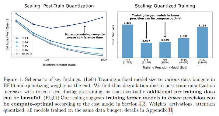
Post-Training Quantization

Core Conclusion: More training tokens are actually harmful!

Let’s explain this seemingly counterintuitive conclusion in detail. In post-training quantization scenarios, we need a pre-trained model checkpoint for quantization to reduce computational overhead during inference. However, quantization inevitably brings model performance loss! Therefore, we can define how much loss quantization actually introduces by using the performance difference between the quantized model and the original model on the same downstream validation set to quantitatively measure how much loss the quantization method brings to the model.

Specifically, the Chinchilla Scaling Law tells us that during the model pre-training phase, the training loss follows this Scaling Law:

where $N$ is the model parameter count, $D$ is the training token count, and the rest are fitting constants. In this paper’s PTQ Scaling Law, they define adding an additional error term introduced by PTQ to this loss item:

Now the question is what factors the additional term $\delta_{\text{PTQ}}$ relates to. Through multiple experiments, the author team obtained this formula:

This formula may seem somewhat abstract, so we can interpret it qualitatively:

The additional loss brought by PTQ is related to three factors: model parameter count $N$, model training token count $D$, and the precision format $P_{\text{post}}$ used:

• The larger the model parameter count, the smaller the additional loss brought by PTQ. This indicates that larger models are relatively less affected by quantization precision loss;
• The more training tokens the model has, the greater the additional loss brought by PTQ. This is also one of the core conclusions of this paper’s section - if a pre-trained model receives more token training, the precision loss it experiences from quantization will be greater;
• The lower the quantization precision used, the greater the additional loss brought by PTQ, following an exponential relationship. This indicates that under the same conditions, the additional loss from x-bit quantization, after taking the logarithm, has a linear relationship with the bit count x.

Specific experimental images and fitting processes can be found in the original paper and won’t be elaborated here. Note that here, the greater additional loss brought by PTQ focuses on the difference value. That is to say, for models of the same size, a checkpoint trained on 1T tokens will definitely be stronger than one trained on 100B tokens, and when both are quantized simultaneously (such as INT4 quantization), the 1T token checkpoint will still be stronger than the 100B token checkpoint! However, the 1T token checkpoint will experience greater degradation compared to the full-precision model than the 100B token checkpoint will!

Quantization Aware Training

Core Conclusion: It’s not necessarily better to train with lower bit precision; 2-bit/1-bit training settings are very likely suboptimal solutions.

In the training phase, the author team also builds upon the original Scaling Law. The original Scaling Law:

is modified to:

The core concept of the author team is that during quantization-aware training, the concept of “effective weight parameter count” can replace the weight parameter count in the original Scaling Law to calculate the training loss. During quantization-aware training, quantization of weights, activations, and attention (KV in the original paper) all bring greater losses. The authors’ experiments found that their effects on the final loss are independent, and the final effects can all be summarized under the concept of effective weight parameter count. Specifically, the authors proposed a method for calculating effective weight parameter count:

Looking at this formula directly is also somewhat abstract. Qualitatively speaking, weights, activations, and attention each control a multiplicative factor for the original parameter count N. Quantizing each item separately will affect the final effective weight parameter count $N_{\text{eff}}$, making the final effective weight parameter count $N_{\text{eff}}$ less than N, thereby increasing the final training error. For each multiplicative factor, it can be seen that they are only related to the quantization precision P of weights, activations, or attention, and follow an exponential relationship. However, weights, activations, and attention have different sensitivity levels to precision, so the formula uses three different sensitivity coefficients $\gamma$ to indicate these relationships, and these coefficients are all fitted from experiments.

In addition to this core conclusion, the authors also proposed some other suggestions regarding QAT. For example, if you want to train models with low precision while the total computational budget is fixed, it is recommended to prioritize expanding the parameter count before considering expanding the training token count.

When considering the training token count N, model scale D, and precision P simultaneously, the calculation of optimal pre-training precision is independent of the total computational budget. For example, 16-bit contains many redundant bits, while 4-bit requires significantly expanding the model scale to maintain training stability. The fitting results in the paper indicate that 7-bit to 8-bit precision achieves the optimal balance between computational efficiency and model performance.

For models that require training with large amounts of tokens and are in an obvious overfitting state, low-precision formats are not suitable during training.

Summary

The authors summarize their findings from these two parts as their proposed Scaling Law for Precision:

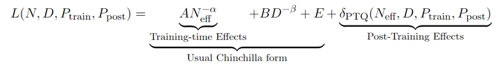
Based on this, the author team reiterates two important points: first, excessive tokens during the pre-training process are likely to cause negative effects during post-training quantization; second, regarding the question of what precision to use during the pre-training phase, the widely-used 16-bit format and the currently highly-hyped extremely low-precision formats such as 4-bit, 2-bit, or even 1-bit formats are not necessarily optimal solutions.

The authors also acknowledge certain limitations of their work: 1) testing only on fixed model architectures; 2) due to system limitations, they were unable to observe the speed advantages brought by low-precision formats; 3) only considering model loss without taking downstream task metrics into account. In my opinion, this paper has other limitations as well, even relatively serious drawbacks:

• Their experimental scale is limited to models of up to 1.7B parameters, with a maximum of 26B tokens trained. Given current LLM development trends, this scale is clearly somewhat small, making one wonder whether this pattern can seamlessly scale to current mainstream model sizes.

• All their experiments are limited to the Dolma 1.7 dataset, with identical training strategies and hyperparameter settings. While it’s admittedly demanding to ask them to conduct more experiments in this regard, considering the first limitation of insufficient scale, along with the complexity of current mainstream LLM training frameworks from various companies, the scalability of this Scaling Law becomes further questionable.

• Looking at results from other Scaling Law studies, the conclusion in this paper that 7-8bit might be optimal would likely be replaced by 4bit in other studies. While this conclusion is somewhat after-the-fact, from an overall perspective of several papers, the method of fitting the QAT loss formula in this paper does not consider the influence of other parameters such as training tokens or quantization granularity on this loss, which indeed has some shortcomings.

In summary, this work published in November 2024 is indeed one of the pioneering works in the quantization Scaling Law field, and their mathematical summary of all conducted experiments is quite comprehensive and complete (though the scaling effects on larger model sizes may not have been verified). It serves as a good foundation for friends who want to further explore Quantization Scaling Laws for additional research.

Low-Bit Quantization Favors Undertrained LLMs: Scaling Laws for Quantized LLMs with 100T Training Tokens (ACL 2025)

Low-Bit Quantization Favors Undertrained LLMs: Scaling Laws for Quantized LLMs with 100T Training Tokens
arxiv.org/abs/2411.17691

This paper comes from the University of Virginia and Tencent AI Lab, with conclusions very similar to the previous paper but described in a more vivid and specific manner. Unlike the previous paper, this paper focuses primarily on Post-Training Quantization.

The core point of this paper is: low-bit quantization favors undertrained LLMs, meaning: small models trained with more tokens have greater error during inference quantization; large models trained with fewer tokens have smaller error during inference quantization.

In Figure 1, the authors show the (fitted) Scaling Laws for 2-bit/3-bit/4-bit respectively. Taking 2-bit as an example, we can see two important conclusions:

• With the same model parameters, as the number of training tokens for the pre-trained model increases, the loss brought by PTQ also increases accordingly
• With the same number of training tokens for the pre-trained model, larger models are less affected by PTQ, meaning the additional loss brought by PTQ is smaller

It’s worth noting that the horizontal axis in these figures reaches the terrifying scale of 10^14, i.e., 100T tokens. Obviously, the authors did not actually train this many tokens, but rather fitted through Scaling Laws.

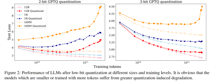
Figure 2 shows the actual experimental situation for the authors. Taking the right figure’s 3-bit GPTQ quantization as an example, the light-colored curves represent the normal training loss curve decline, while the dark-colored corresponding curves indicate the loss situation after PTQ quantization of the corresponding checkpoint. It can be seen that smaller models, or models trained with more tokens, perform worse after quantization. Similar phenomena are even more severe in 2-bit quantization scenarios.

Regarding this discovery, the author team vividly uses the concept of “training sufficiency” to describe whether an LLM is susceptible to quantization effects. Smaller models, or models trained with more tokens, all belong to the case of relatively sufficient training. So this is what the title says: quantization favors undertrained models, which either have more parameters or have received insufficient training tokens. This conclusion is actually consistent with the conclusion of the first Scaling Law paper.

In horizontal comparison with other Quantization Scaling Law articles, the limitations of this paper lie in: first, only considering post-training quantization (Post-Training Quantization), and second, treating the performance degradation caused by post-training quantization (referred to as QiD in the paper) as the sole metric for measuring performance. However, in practical applications, this metric is not comprehensive and cannot fully reflect the performance of quantized models. Other evaluation metrics such as downstream task accuracy should also be considered.

Compression Scaling Laws: Unifying Sparsity and Quantization

Compression Scaling Laws: Unifying Sparsity and Quantization
arxiv.org/abs/2502.16440

This work comes from Google DeepMind, mainly targeting Quantization-Aware Training Scaling Law, and more specifically focusing on weight-only scenarios. The main text and experiments of this work are relatively few, so we’ll quickly go through their core conclusions here.

Similar to the first Scaling Law paper, the author team proposes modifying the original Scaling Law:

to:

That is, using the concept of “effective weight parameter count” to replace the weight parameter count in the original Scaling Law. Compared to the first Scaling Law paper, here the authors further clarify that the effective weight parameter count is the original parameter count multiplied by an effective coefficient $\text{eff}(C)$, where C is the quantization method. This coefficient is independent of other influencing factors, and once the quantization method is determined, this effective coefficient becomes a constant.

This modeling approach is indeed more concise (though whether this assumption is accurate in practical scenarios remains to be verified). Under this modeling approach, the core conclusion of the author team is:

• When only performing weight quantization (weight-only quantization), the author team found that the effective coefficient is very close to 1, indicating that quantization has very little impact and can maintain good accuracy even under 4-bit quantization.

• When quantizing both weights and activations, when the quantization bits drop below 4-bit, model accuracy rapidly degrades. This suggests that 4-bit quantization may be the optimal solution for full-model quantization.

Compared to other papers, this paper has more limitations, and the biggest drawback may lie in its theoretical modeling of Quantization Scaling Law itself, which is somewhat lacking. However, it reminds us again that model quantization is not necessarily better with lower bit precision.

Scaling Law for Quantization-Aware Training ⭐

Scaling Law for Quantization-Aware Training
arxiv.org/abs/2505.14302

This paper comes from the University of Hong Kong and ByteDance’s Seed team, systematically and comprehensively studying the Scaling Law in quantization-aware training processes, particularly conducting in-depth research on 4-bit training (W4A4).

A significant difference between this work and the above works is that the mathematical form of the proposed Scaling Law is quite different. Apologies for having to present formulas again, but there’s no way around it since to better understand this paper, we must first understand the Scaling Law they propose. The original Chinchilla Scaling Law:

The improvements made by the first Scaling Law (QAT section) and the third Scaling Law are:

The advantage of this approach is that it can directly use the equivalent model parameter count to replace the parameter count in the original formula, but the disadvantage is that it does not consider the influence of other factors on the loss in quantization training. In this paper, these other factors include the training token count and the quantization granularity used. Therefore, the author team believes it would be better to directly add a QAT-related loss term directly to the original loss:

This term represents the additional loss introduced by QAT. This idea is actually quite direct and consistent with the PTQ additional loss introduced in the first work. The advantage of this approach is that it can more comprehensively reflect the influence of more factors on this additional loss.

Through extensive experiments, the authors propose the fitting formula for this additional QAT loss term:

where D is the training token count, G is the quantization granularity, and N is the model parameter count. The paper proposes that the loss brought by QAT (Quantization-Aware Training) is related to three key factors:

• The larger the training data volume, the greater the loss brought by QAT, showing a positive correlation. This indicates that when models are trained on more data, their performance is more easily affected by quantization perturbations;
• The larger the model parameter count, the smaller the loss brought by QAT, showing a negative correlation. This indicates that larger models have stronger robustness when facing errors brought by quantization;
• The larger the quantization granularity G, the greater the loss brought by QAT, with a logarithmic growth relationship. That is to say, under the same conditions, as quantization granularity increases, the additional loss increases according to the trend of $\log G$.

Here, let me further explain the concept of quantization granularity G size. If we quantize an entire tensor, this is quite low quantization granularity because it’s definitely not as precise as quantizing after chunking. In this case, we say the quantization granularity G is very large, up to the size of the entire tensor. In block-wise quantization, G directly represents the size of each chunk after partitioning. Therefore, the smaller the quantization granularity, the higher the quantization accuracy, but the computational complexity of the quantization operation will also increase.

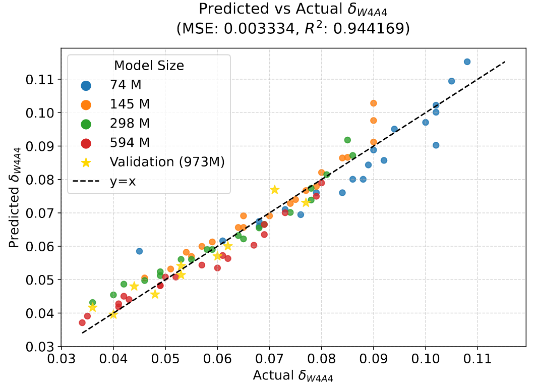
To further explain the above formula with a concrete example, this figure shows the experimental results of 4-bit full quantization (W4A4).

Figure (a): Training with the same 100B tokens, different colored curves represent different quantization granularities. It can be seen that all curves follow the pattern where the larger the model size, the smaller the final $\delta_{W4A4}$. Here, $\delta_{W4A4}$ represents the difference between the final training error of the model trained under W4A4 conditions and the training error of the full-precision model.

Figure (b): With the same 594M model size, different colored curves represent different quantization granularities. It can be seen that all curves follow the pattern where the more training tokens used, the larger the final $\delta_{W4A4}$.

Figure (c): With fixed training of 594M model and 100B tokens, it can be observed that as the quantization granularity (i.e., Group size on the horizontal axis in the figure) decreases exponentially, the final $\delta_{W4A4}$ shows a linear downward trend.

In addition to this, this paper carefully studied how to decouple W and A in W4A4. The first question is: is the additional loss caused by jointly quantizing W and A equivalent to the sum of the loss from quantizing W alone plus the loss from quantizing A alone? The authors found through experiments that the following relationship indeed holds:

That is, the influence of separately quantizing weights and separately quantizing activations on QAT loss is indeed independently additive. Then, what is the relationship between the influence of separately quantizing weights and separately quantizing activations on QAT loss and the three influencing factors N, D, G mentioned above? How do their sensitivities differ? The author team obtained the following conclusions through experiments:

• As the model scale N increases, $\delta_{W4A16}$ decreases faster than $\delta_{W16A4}$, indicating that during the process of model expansion, the impact of weight quantization on accuracy decreases more rapidly.

• As the training token count D increases, $\delta_{W4A16}$ increases faster than $\delta_{W4A16}$, indicating that the influence of weight quantization error on overall loss becomes more significant as the data volume increases.

• Regarding quantization granularity G, $\delta_{W16A4}$ is more sensitive to changes, meaning that activation quantization is more susceptible to the coarseness of granularity than weight quantization.

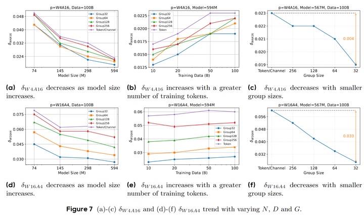
Figure 7 is similar to Figure 4, separately analyzing the relationship between $\delta_{W16A4}$ and $\delta_{W4A16}$ with respect to N, D, and G, showing that their sensitivity to these influencing factors is indeed different.

The above conclusions indicate that as the D/N ratio increases, the primary source of quantization error gradually shifts from activations to weights. However, even at higher D/N values and finer granularities (such as G=32), $\delta_{W16A4}$ remains larger than $\delta_{W4A16}$, and the gap between the two further widens under coarse granularities. This indicates that in W4A4 quantization, activation quantization error is typically the dominant factor, highlighting the importance of optimizing activation quantization for improving W4A4 quantization performance.

Since activation quantization is the dominant factor, the author team further investigated what causes $\delta_{W16A4}$ to be larger. The author team found that outliers in the output layer of each transformer layer (referred to as the FC2 Proj layer in the paper) significantly affect quantization performance. Therefore, special processing of the FC2 Proj layer input, such as using mixed-precision quantization or targeted outlier suppression, is crucial for achieving optimal performance in low-bit QAT.

In summary, this paper provides a comprehensive and detailed analysis of low-bit QAT, particularly 4-bit QAT. Both from a theoretical analysis perspective and experimental completeness, it is highly persuasive, and the paper also introduces some practical experiences in the actual model training process based on the derived Scaling Law, such as special processing for the FC2 Proj layer to reduce activation quantization errors.

However, the downside is that the experiments in this paper are limited to models of up to 595M parameters, with a maximum of 100B training tokens. While fitting Scaling Laws is indeed a very expensive task, we also look forward to quantization series work achieving substantial breakthroughs at larger scales.

Scaling Laws for Floating-Point Quantization Training (ICML 2025)

Scaling Laws for Floating-Point Quantization Training
arxiv.org/abs/2501.02423

This paper comes from the Tencent HunYuan team, University of Macau, Chinese University of Hong Kong, and others, still focusing on in-training quantization. The highlight is the introduction of Scaling Law regarding floating-point quantization, incorporating the key parameters of floating-point quantization—exponent bit count E and mantissa bit count M—into the Scaling Law, making this theory more complete in the field of floating-point quantization.

Based on the Chinchilla Scaling Law, similar to the above Scaling Law papers, they also add a floating-point QAT quantization compensation term after the Loss item. They named their proposed Scaling Law the Capybara Scaling Law (lol), reasoning that when the model size is fixed, adding more training tokens does not bring better quantization results (this conclusion has been found in this series of Scaling Laws), and the situation where greater “pressure” leads to worse results is just like a capybara—applying pressure to it actually backfires.

The Capybara Scaling Law proposed in the article is as follows:

where the first three terms are the original Chinchilla Scaling Law, and the subsequent compensation term: D is the training token count, N is the model size, B is the block size in block-wise quantization, i.e., quantization granularity. The trends of these three variables are actually identical to the previous Scaling Law. In addition to these three variables, the denominator also includes the exponent bit count E and mantissa bit count M in floating-point quantization. Larger E and larger M represent using more bits for quantization, which naturally brings smaller errors.

We won’t elaborate on the specific experimental settings and fitting calculation processes here, and will directly show some key findings from this article:

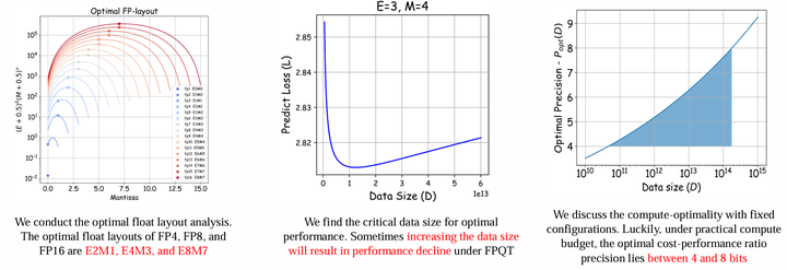
First, the authors investigated the quantization training effects of various floating-point formats and discovered the optimal E, M allocation under fixed total bit count. Specifically, the optimal formats for FP4, FP8, and FP16 are E2M1, E4M3, and E8M7 respectively. The BF16 format commonly used in deep learning today happens to have the E8M7 allocation strategy for 16 bits (1 sign bit + 8 exponent bits + 7 mantissa bits), while the normal FP16 format allocation strategy is E5M10. The FP8 format used in the Deepseek-V3 paper during model training happens to be E4M3 format, and the FP4 format used in the paper “Optimizing Large Language Model Training Using FP4 Quantization” during model training also happens to be E2M1 format.

Secondly, the author team found that under fixed model size and bit count, blindly increasing the number of training tokens ultimately leads to a decline in model performance. Further, the authors proposed the following formula to estimate this optimal data quantity threshold:

Finally, the author team also carefully discussed what the optimal training setup should be under a fixed total computational budget. The entire mathematical reasoning process is quite complex, but in general, for a computational budget that would be used in practical scenarios, 4-bit to 8-bit would be an optimal quantization strategy.

The limitations of this paper also largely remain within the main limitations restricting Scaling Laws: the largest fitting experiment scale reached 679M model size with 100B training tokens, and verification experiments were also conducted on 1.2B size models. Additionally, this series of experiments was only conducted on traditional Transformer models.

Summary

In the Quantization Scaling Law field, a general consensus is that whether for training or inference, blindly reducing bit count is not the optimal solution. Researchers should not pursue so-called research novelty by constantly hyping how many bits they have quantized some model to, but rather spend more effort considering how to actually utilize low-bit quantization in practical applications.

Quantization Scaling Law also tells us that larger models are more suitable for low-bit quantization. Under fixed training costs, training a larger model with lower precision often performs better than training a smaller model with higher precision. Additionally, the scale of model training corpora needs to be considered. If the training budget is sufficient and one wants to train many tokens, even to the point of overfitting the model, then low-bit formats are not suitable in such cases.

Delving deeper into the quantization methods themselves, we can further discover from Quantization Scaling Law that quantization granularity size and E/M allocation methods during floating-point quantization will all affect the final model performance. This tells us that if we want to use low-precision formats for model training, we need to carefully fit and determine this series of parameters before formal training to ensure that the final model’s performance doesn’t experience severe degradation.

Unconsciously, I’ve written over ten thousand words, showing that truly understanding the articles within a small series still requires considerable effort. The paper interpretation series will continue to be updated, and everyone is welcome to exchange thoughts!