Stop Wasting Your Pre-trained Checkpoints: Orthogonal Growth Saves You 10%+ Compute
Published:
This blog is also available in Chinese version: https://zhuanlan.zhihu.com/p/2055327145866552638
Detailed Paper Interpretation of “Beyond Sunk Costs: Boosting LLM Pre-training Efficiency via Orthogonal Growth of Mixture-of-Experts”
If you’ve worked on large-scale pre-training, you’ve probably been in this situation: you spent weeks (or months) training a model. It’s converged, it performs well at its current size. But now you need something bigger. Scaling laws tell us that model performance correlates with parameter count—more layers, more parameters, better downstream results. What do you do? The standard answer in the industry is: throw away that checkpoint and train a larger model from scratch. Simple enough, but all those FLOPs you invested? Gone.
In practice, the LLM development pipeline frequently produces smaller models—trained for system validation, hyperparameter tuning, or preliminary evaluation. These models are often well-trained, but get discarded once the goal shifts to larger-scale training. Can we recycle these checkpoints and save the “sunk cost”? That is, grow a well-trained model into a larger one, inheriting everything it has already learned? This is the starting point of this paper. Based on this motivation, we developed our growth methods and conducted detailed experimental analysis, published as: Beyond Sunk Costs: Boosting LLM Pre-training Efficiency via Orthogonal Growth of Mixture-of-Experts
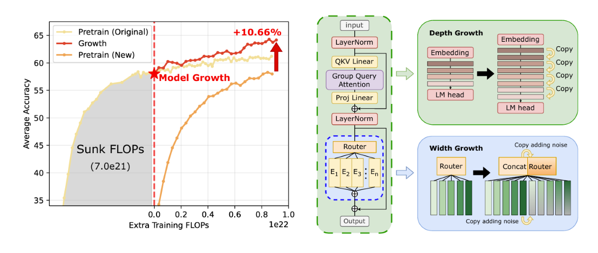
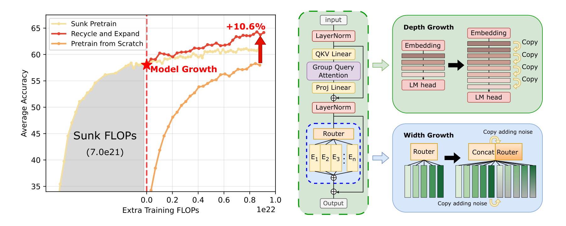 Figure 1. Overview of the orthogonal growth framework: (left) efficiency comparison between the grown model and training from scratch under equal extra compute; (right) illustration of depth growth (Interposition) and width growth (expert duplication).
The left panel shows the result: our grown model (17B→70B) achieves 10.6% higher accuracy than a 70B model trained from scratch with the same extra compute. The right panel shows the two growth directions—adding layers (depth) and adding experts (width).
Paper: Beyond Sunk Costs: Boosting LLM Pre-training Efficiency via Orthogonal Growth of Mixture-of-Experts
Background and Motivation
Model growth simply means: take a trained model, expand its architecture to have more parameters, then keep training. The idea is not new—Net2Net dates back to the CNN era, Bert2Bert and StackBert appeared in the BERT era, and ViT had LiGO and LEMON. In the LLM era, LLaMA-Pro, Solar 10.7B, and FLM-101B have done similar things. But prior work shares two common limitations:
- Many only grow models early in training (before convergence), leaving the question of “how to grow a well-trained model” unanswered
- Systematic study of MoE architecture growth is lacking. MoE has unique expert structures that cannot simply reuse dense model growth methods
There is also a related but distinct direction called MoE Upcycling: converting a dense model into MoE. This is fundamentally different from what we do. In upcycling, the router is randomly initialized and requires heavy noise (50%+) to drive expert differentiation. We are expanding an existing MoE model where the router is already well-trained, requiring a completely different noise regime.
For MoE models, there are two natural expansion axes:
- Depth: duplicate transformer layers to make the model deeper
- Width: duplicate experts to give each layer more computational capacity
Intuitively, the simplest approach to model expansion is direct copying. But how you copy turns out to matter a great deal when the base model has been trained extensively and fully converged. The following sections detail each direction:
Depth Growth: Stacking vs. Interposition
Two ways to double your layers
Say your model has layers $l_1, l_2, \dots, l_n$. If you want to double the depth, there are two straightforward approaches:
Stacking: the widely-used baseline: \(M_{\text{stack}} = l_1, l_2, \dots, l_n, \; l_1, l_2, \dots, l_n\)
Concatenate the entire model with a copy of itself. LLaMA-Pro, Solar 10.7B, Staged Training and other prior work use this.
Interposition: our approach: \(M_{\text{interp}} = l_1, l_1, \; l_2, l_2, \; \dots, \; l_n, l_n\)
Duplicate each layer right next to itself. Same total parameter count, very different structural outcome.
If your model hasn’t been trained much, both work about equally well. But for a well-converged model? Our paper will show in detail that the gap is dramatic.
Why interposition works better: the weight norm story
We discovered an interesting phenomenon during our experiments. When we plotted the per-layer weight norms of various well-trained LLMs, they all exhibit a common pattern: norms increase monotonically from shallow to deep layers. These models include our own 3B and 17B, as well as open-source models like Deepseek-v2-Lite, Qwen1.5-MoE, Mixtral-8x7B, Hunyuan, Dots-LLM1, and GroveMoE.
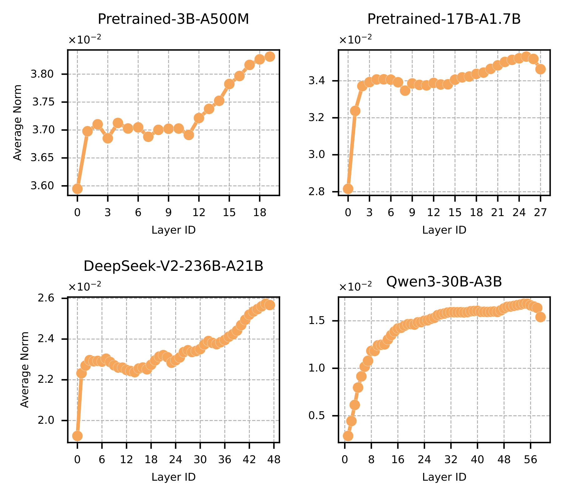 Figure 2. Per-layer weight norm distributions across four representative MoE models (our 3B, our 17B, and two open-source models). All exhibit a universal monotonically increasing pattern from shallow to deep layers.
Specifically, we compute the average Frobenius norm (flatten the 2D tensor, compute L2 norm) of all expert weight matrices per layer, normalized by the square root of the parameter count. This metric shows the same trend across architectures and scales. The appendix includes norm distributions for additional open-source models (Deepseek-v2-Lite-16B, Qwen1.5-MoE-14.3B, Mixtral-8x7B, Hunyuan-A13B, Dots-LLM1-142B, GroveMoE-33B), all confirming the same conclusion.
This pattern has a theoretical explanation. Marion et al. (ICLR 2024) proved that ResNets trained with gradient flow are implicitly regularized toward neural ODEs, meaning the per-layer transformation $x_{l+1} = x_l + f_l(x_l)$ should form a “smooth” sequence. Wang et al. (2024, DeepNet) further showed that stable deep training requires controlling residual contributions across layers. Together, this increasing norm profile is a structural signature of “healthy convergence”.
Now think about what each growth method does to this smooth profile:
- Stacking: you go from layer $n$ (high norm) immediately back to layer 1 (low norm). This creates a cliff—a massive discontinuity. The model has to spend training budget repairing it.
- Interposition: every layer stays next to its neighbor. The profile stays smooth. Nothing to repair.
We quantified this effect. At the growth boundary (layer 19→20 in our 20-layer model), stacking creates a norm jump of about 10× the typical inter-layer variation:
| Layer | Base Original | Stack @init | Stack +16k steps | Interposition @init | Interposition +16k steps |
|---|---|---|---|---|---|
| 0 | .0323 | .0323 | .0352 | .0323 | .0349 |
| 10 | .0336 | .0336 | .0363 | .0337 | .0363 |
| 19 | .0356 | .0356 | .0373 | .0336 | .0362 |
| 20 | — | .0323 ↓ | .0367 ↓ | .0336 | .0362 |
| 30 | — | .0336 | .0373 | .0347 | .0370 |
| 39 | — | .0356 | .0373 | .0356 | .0376 |
Look at layers 19→20: Stacking initialization drops from .0356 to .0323, and after 16k training steps the gap shrinks but persists (.0373→.0367). Interposition remains smooth throughout. The stacking model spends its first few thousand training steps repairing this cliff, effectively wasting compute.
Performance gap
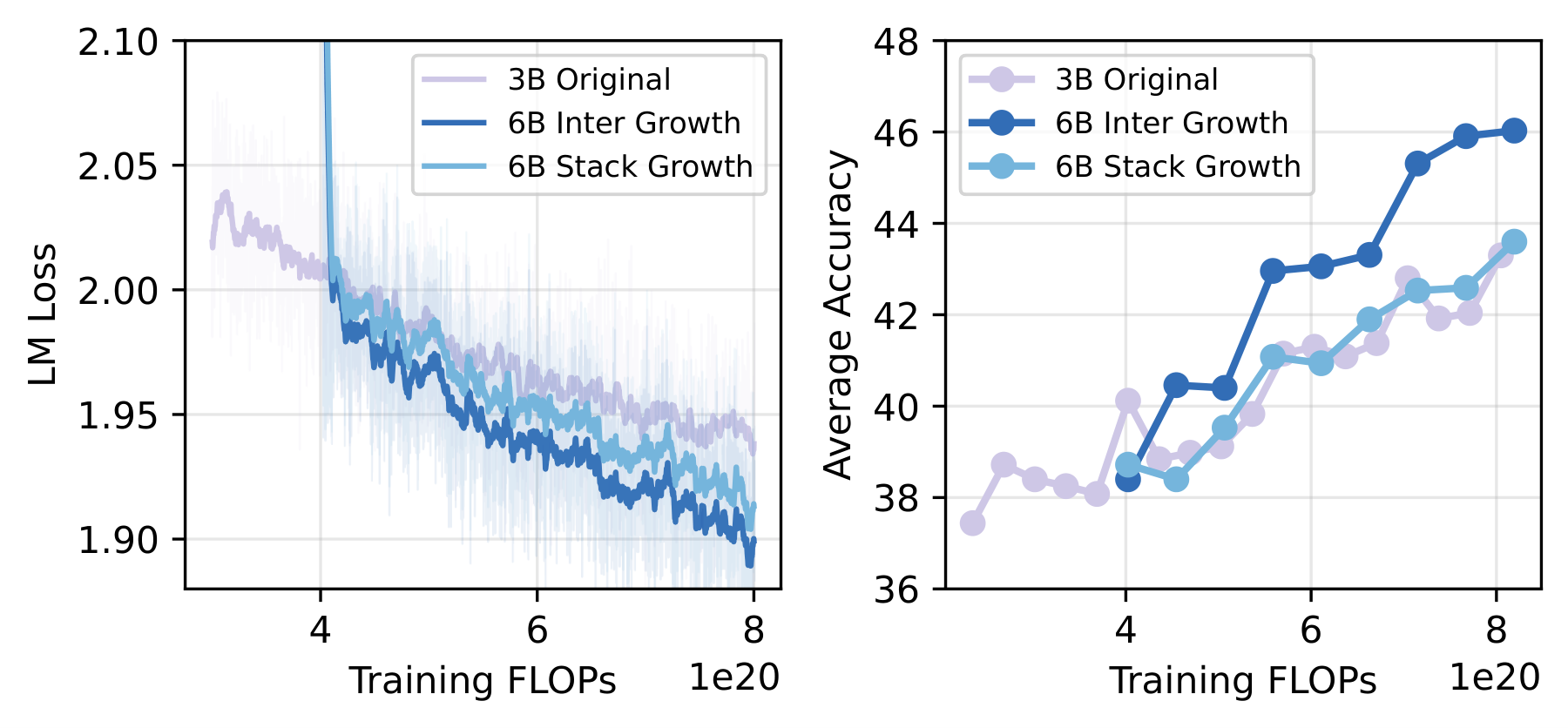 Figure 3. Training loss and downstream accuracy for Interposition vs. Stacking on 3B→6B growth (k=2). Interposition consistently achieves lower loss and higher accuracy throughout continued training.
Beyond the theoretical analysis, we provide end-to-end experiments to substantiate this point. Using a 3B MoE model (0.7B activated parameters), we grow it to a 6B MoE model using both Interposition and Stacking. With FLOPs as the x-axis (fair comparison, since the grown model is larger), Interposition consistently shows lower loss and higher accuracy, and this advantage persists throughout training.
Here we use a fixed growth hyperparameter $k=2$, consistent with most model growth papers which do not treat $k$ as a tunable or learnable parameter. However, we argue that Interposition’s advantage extends to larger $k$. For example, when $k=4$, expanding 20 layers to 80:
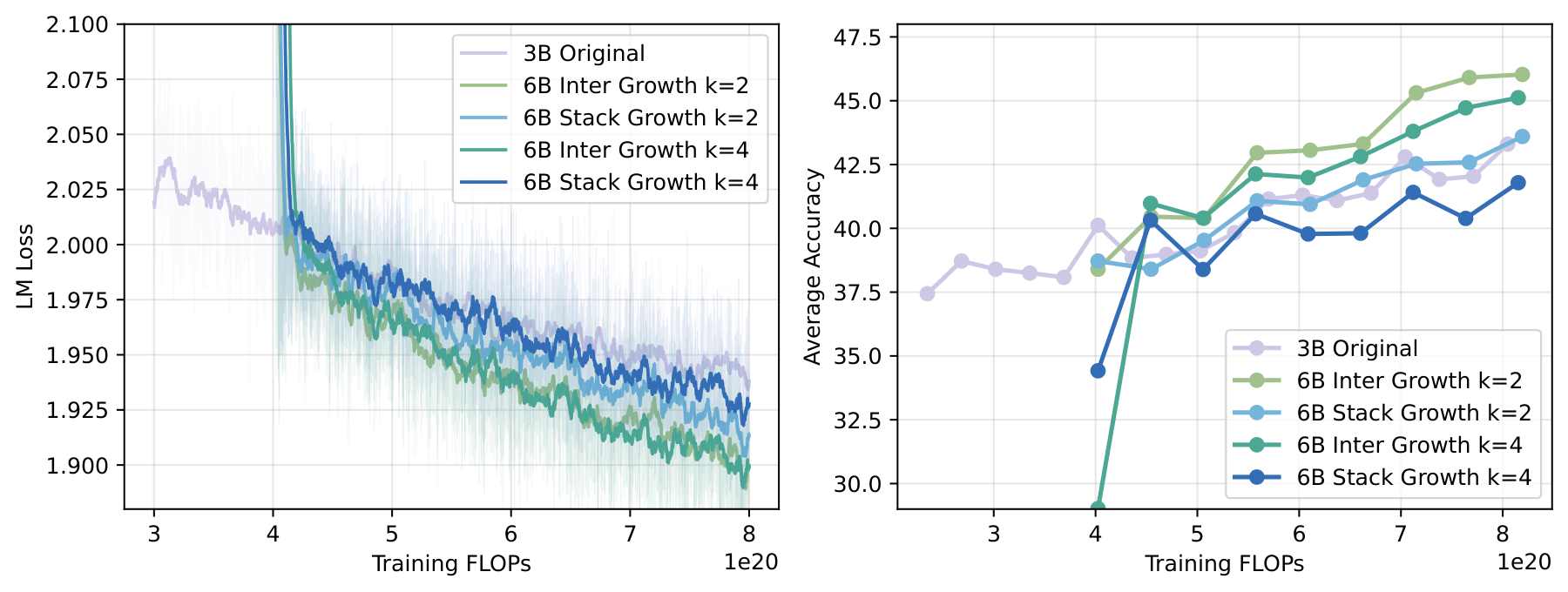 Figure 4. Interposition vs. Stacking under growth factors k=2 and k=4. The performance gap widens at larger expansion factors, consistent with the theoretical prediction.
The advantage not only persists but grows larger. This aligns with theory: larger $k$ means Stacking creates a more severe “rise-then-drop” norm pattern with repeated cliffs from deep-layer norms jumping back to shallow-layer norms, while Interposition always maintains smoothness. So for larger expansion factors, Interposition’s advantage becomes even more pronounced.
When should you use Interposition? Quantitatively finding the boundary
Does interposition always beat stacking? Intuitively not—if the model has barely started training, norms should still be uniform (random initialization), and the two methods should perform similarly.
To quantify this boundary, we ran a systematic experiment: using training FLOPs as a progress metric, we take checkpoints from different stages and apply both methods.
Here we introduce a concept: the Chinchilla-optimal FLOPs, denoted $F_c$. For MoE models, we approximate using activated parameters (following Switch Transformer): $F_c \approx 6 \cdot N_a \cdot (20 N_a)$. For our 3B model ($N_a$ = 700M), $F_c \approx 5.88 \times 10^{19}$. In practice, small models are often “overtrained” (trained far beyond $F_c$).
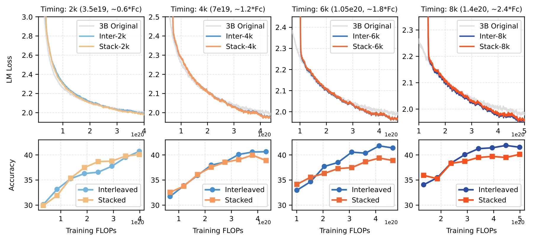 Figure 5. Interposition vs. Stacking at different growth timings (varying pre-training FLOPs budget). Interposition’s advantage becomes clear once training exceeds ~1× Chinchilla-optimal FLOPs.
The training results show that once training FLOPs exceed approximately $1 \times F_c$, Interposition starts clearly winning. Before that, the two methods are similar.
Why this boundary? We can directly observe the norm pattern formation:
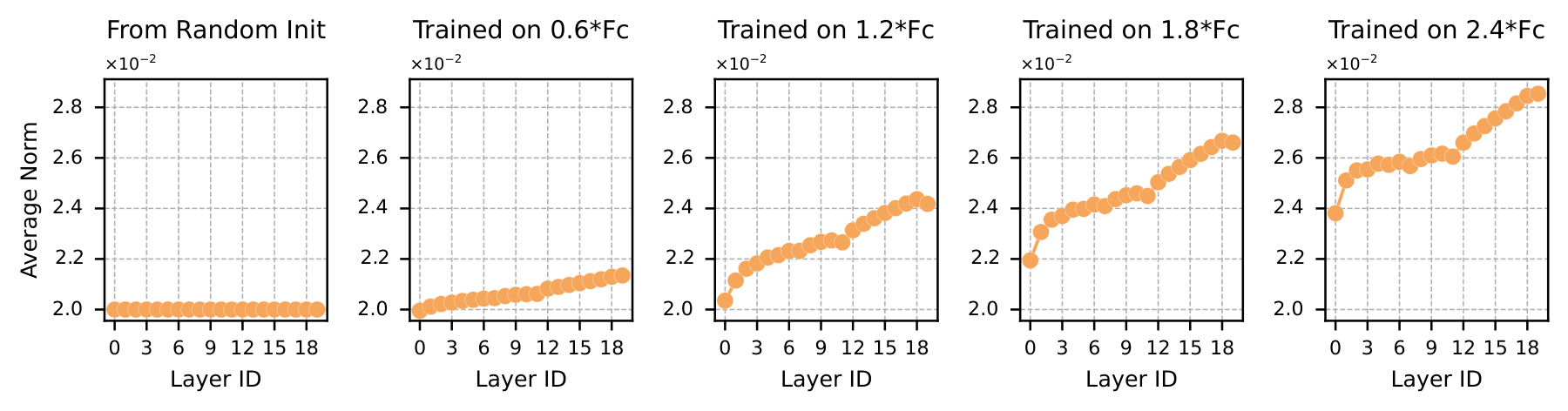 Figure 6. Evolution of per-layer weight norm during 3B model training (step 0 to 48k). Norms begin uniform and stabilize into a monotonically increasing pattern around 4k steps (~1.2×F_c), marking the onset of Interposition’s advantage.
At initialization, norms are flat (all layers initialized from the same Gaussian, std=0.02). Around 4k steps ($\approx 1.2F_c$), the increasing pattern stabilizes. This is exactly when Interposition starts winning. In other words: the formation of the increasing norm pattern marks the boundary where Interposition begins to outperform Stacking.
In practice, nearly all modern LLMs are “overtrained” (trained far beyond $F_c$), so Interposition is generally the more suitable choice.
Width Growth: Duplicating Experts with a Small Perturbation
For MoE models, the other growth direction is expert duplication. Our approach:
- Double the total expert count ($E → 2E$)
- Double the activated expert count ($k → 2k$)
- Initialize new experts as copies of the originals, with a small amount of noise added
Specifically, for the output of an original MoE layer:
\[F(x) = \sum_{i \in \mathcal{T}} g_i(x) f_i(x), \quad \mathcal{T} = \text{Top}_k(g(x))\]where $f_i$ is the $i$-th expert, $g(x) \in \mathbb{R}^E$ is the gating weight from the router. We duplicate both expert weights and their corresponding router weights, then add Gaussian noise: $\epsilon \sim \mathcal{N}(0, (\alpha \sigma_{\text{orig}})^2)$, where $\sigma_{\text{orig}}$ is the standard deviation of the original parameters.
The noise might seem like a minor detail, but it is critical. With exact duplication ($\alpha = 0$), all new experts see identical gradients from the router, making subsequent differentiation impossible. A small perturbation ($\alpha = 0.01$, i.e., noise std = 1% of original parameter std) gently breaks this symmetry, allowing different experts to gradually specialize during training.
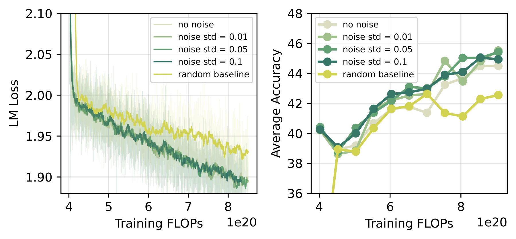 Figure 7. Ablation on perturbation scale α for expert duplication. α=0.01 is optimal; exact copy (α=0) causes symmetry deadlock preventing expert specialization, large noise destroys learned router weights, and random initialization of new experts performs worst.
A few points worth noting:
- Small noise ($\alpha=0.01$) yields about 1% accuracy improvement over exact duplication. Loss is similar, but downstream task performance improves meaningfully
- Too much noise is harmful, which is very different from upcycling dense models to MoE. Upcycling requires 50%+ perturbation because the router is randomly initialized (see Sparse Upcycling, OLMoE). We already have a well-trained router, so large noise destroys what has been learned
- Randomly initializing new experts (keeping originals, the random baseline in the figure) performs notably worse, confirming that the benefit comes from knowledge inheritance rather than simply breaking symmetry
Why double both E and k?
We also conducted a routing variants ablation study to justify this design choice:
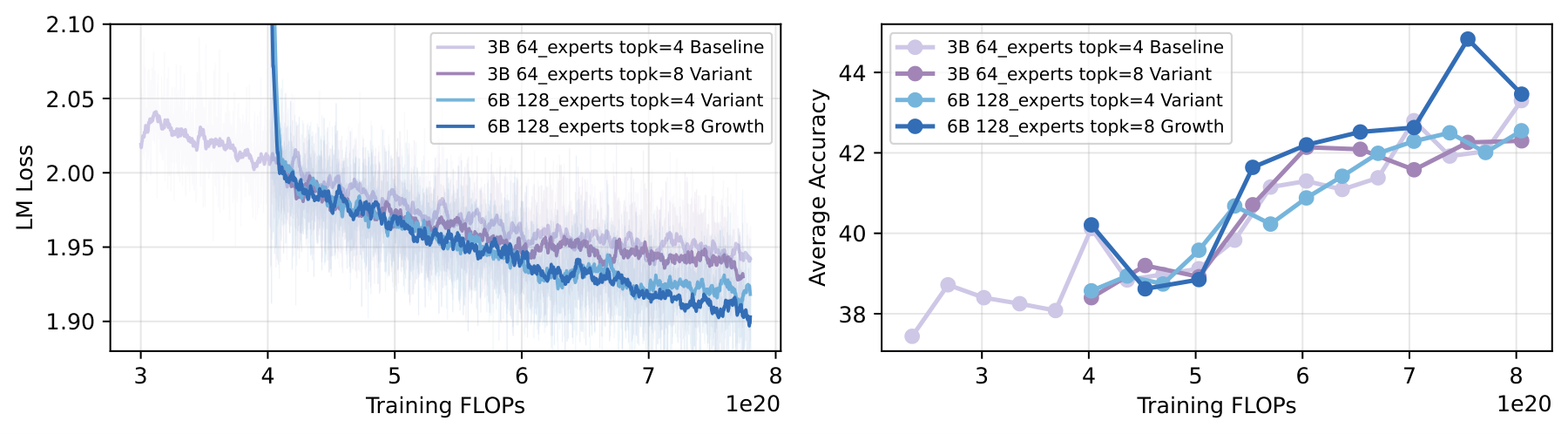 Figure 8. Width growth routing variants: doubling both E and k (ours, 6B-A900M/top-8) vs. E-only doubling (6B-A700M/top-4, fixed activation count) vs. k-only doubling (3B-A900M/top-8, fixed expert count). Scaling capacity and computation together is necessary for optimal performance.
Three configurations compared:
- 6B-A900M (top-8/128): our approach, doubling both E and k → best performance
- 6B-A700M (top-4/128): only adding experts without increasing activation count (E doubled, k unchanged) → inferior. This shows that expanding capacity without increasing computation is insufficient. Adding more experts while activating the same number per forward pass means new experts do not receive enough training signal
- 3B-A900M (top-8/64): only increasing activation count without adding experts (k doubled, E unchanged) → initially competitive but convergence slows later. This shows that increasing computation under fixed capacity eventually hits a wall. Using more computation on a limited knowledge base yields diminishing marginal returns
The conclusion: effective MoE growth requires capacity and computation to scale together, which is why we choose to double both E and k simultaneously.
Orthogonality: Depth and Width Don’t Interfere
Having introduced both width growth and depth growth, a natural question arises: if you grow in both directions, do they interfere? Does doing depth first affect the effectiveness of subsequent width growth?
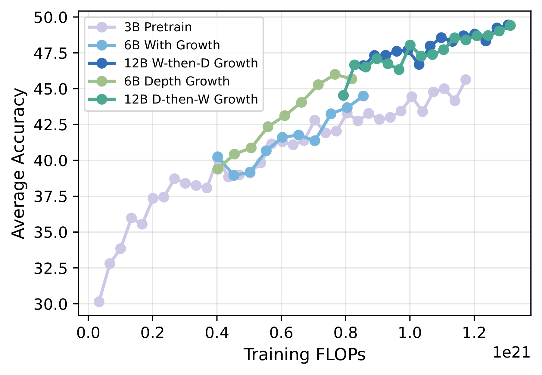 Figure 9. Accuracy comparison across four growth strategies at 12B scale: depth→width, width→depth, depth-only, and width-only. The two combined orderings yield identical results, confirming order independence.
Our experiments demonstrate that the two do not interfere: depth→width and width→depth yield the same final result. We verified this “orthogonality” from four perspectives:
1. Structural orthogonality: Depth growth adds 3280 tensors (all parameters from 16 new layers), width growth adds 3840 tensors (64 new experts × 20 layers). The two parameter sets have zero intersection: depth does not touch any expert, width does not add any layer.
2. Gradient direction orthogonality: Starting from the same base checkpoint, we perform depth growth and width growth separately, extract Adam optimizer first moments (i.e., $m_t = \beta_1 m_{t-1} + (1-\beta_1) g_t$, exponential moving average of gradients), and compute cosine similarity on shared parameters:
| Steps after growth | cos(base, depth) | cos(base, width) |
|---|---|---|
| +2k | 0.031 | −0.003 |
| +4k | 0.039 | 0.022 |
| +8k | −0.001 | 0.027 |
| +16k | 0.016 | 0.038 |
| Both types of growth redirect optimization to directions nearly orthogonal to the pre-growth direction ( | cos | < 0.04), and this orthogonality remains stable throughout 16k training steps. This indicates that growth introduces entirely new learning signals—the model is exploring directions it had never explored before growth. |
3. Weight update divergence: From the same base, after performing depth and width growth separately, we measure the cosine similarity of cumulative weight changes ($\Delta = \theta_{\text{grown}}(t) - \theta_{\text{base}}$) on shared parameters:
| Steps | Overall | Expert FFN | Attention | Embedding |
|---|---|---|---|---|
| +2k | 0.630 | 0.614 | 0.635 | 0.781 |
| +8k | 0.490 | 0.469 | 0.562 | 0.725 |
| +16k | 0.431 | 0.406 | 0.551 | 0.713 |
| +20k | 0.418 | 0.393 | 0.554 | 0.710 |
Expert FFN (the core MoE parameters) diverge fastest (0.614→0.393), while Embedding maintains higher correlation (as expected—vocabulary representations are shared and neither growth type changes the vocabulary). The initial 0.63 can be understood as a brief “recovery period” after growth—both models have just experienced architectural perturbation and are adjusting toward the nearest loss valley, a process with some inherent correlation. But as training progresses, each develops specialized representations, and updates become increasingly uncorrelated.
4. Order independence at 12B scale: On the 12B model (the actual target scale), we verify that models from depth→width and width→depth paths maintain weight cosine similarity consistently > 0.82, with uniform distribution across layers (0.78-0.86) and no local anomalies. Attention parameters show highest consistency (0.953), router lowest (0.807)—as expected, since the router is most sensitive to expert composition, and the two orderings produce subtly different expert distribution structures.
Taken together, these analyses yield a unified conclusion: depth and width growth are approximately orthogonal in both parameter space and optimization landscape, and can be combined in any order without interference.
More Sunk Cost, Better Growth
Next is what we consider the most practically valuable finding: more prior training = better post-growth performance. This conclusion is valuable because practitioners often intuitively worry: can a model that has already fully converged or even started annealing still benefit from growth? Will the marginal returns diminish to near zero?
The experimental design is straightforward: we first train the 3B model to completion (warmup → constant LR → annealing), take 12 checkpoints from different stages (8k to 96k steps), perform depth growth to 6B on each, and give them all the same additional FLOPs budget ($3 \times 10^{20}$ FLOPs). We add a 6B model trained from scratch as a baseline (representing sunk cost = 0).
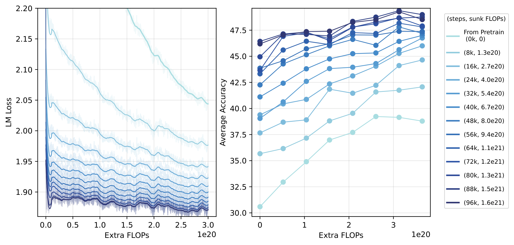 Figure 10. Final evaluation accuracy vs. sunk-cost FLOPs under a fixed extra training budget ($3\times10^{20}$ FLOPs). A strong positive correlation confirms that prior training is fully recycled, not wasted.
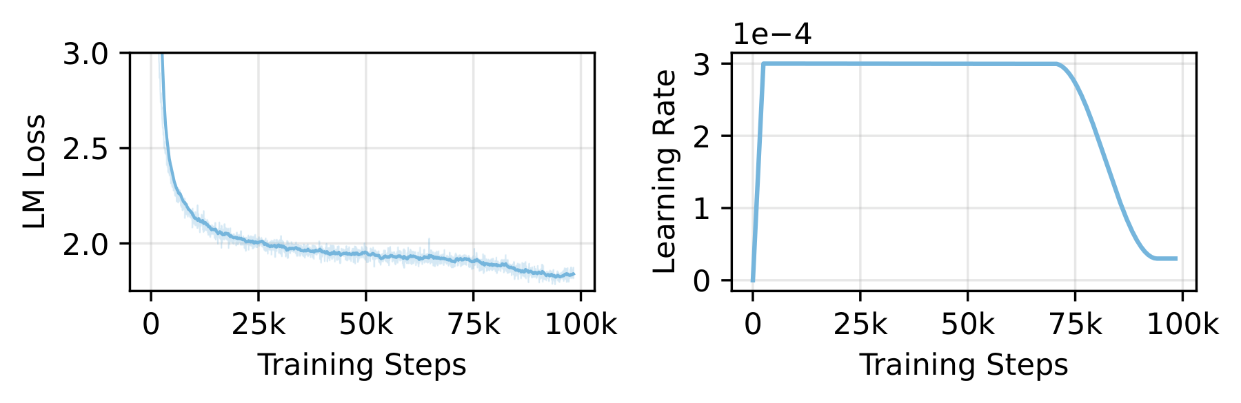 Figure 11. Complete training trajectory of the 3B base model with LR schedule, showing warmup, constant-LR, and annealing phases. Growth checkpoints are sampled across all three stages.
Specific numbers:
| Start Step | Start acc | End acc | Average acc |
|---|---|---|---|
| 0k (from scratch) | 30.59 | 38.79 | 36.29 |
| 8k | 35.67 | 42.07 | 39.09 |
| 16k | 37.66 | 44.65 | 41.19 |
| 32k | 39.05 | 46.75 | 43.34 |
| 56k | 43.86 | 47.37 | 46.15 |
| 80k | 44.95 | 48.76 | 47.43 |
| 96k | 46.19 | 48.52 | 47.82 |
Strong positive correlation—every additional step of pre-training translates into better post-growth performance, demonstrating that model growth genuinely recycles prior compute investment rather than starting over.
Notably, marginal returns diminish after entering the annealing phase (beyond 72k steps). This is because for fair comparison, all grown models use the same constant LR ($3 \times 10^{-4}$) for continued training—which may not be optimal for checkpoints taken from the annealing phase (the LR had already been reduced, then suddenly raised back to constant LR). Practical recommendation: either carefully tune the post-growth learning rate, or preferably grow from constant-LR phase checkpoints.
Fixed total budget: growth vs. scratch
The above experiment fixes the “extra” budget. A sharper question: if the total FLOPs are fixed, is it better to train a large model from scratch, or train a small one first and then grow it?
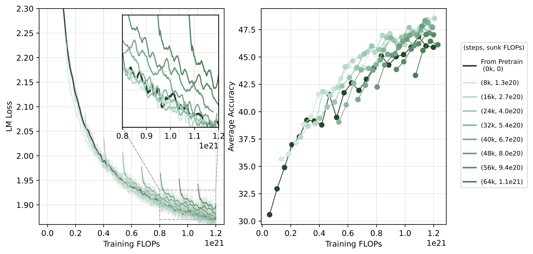 Figure 12. End accuracy and average accuracy under a fixed total FLOPs budget for different growth timings. Growing at ~16k steps is optimal; too-late growth leaves insufficient budget for the larger model to converge.
| Start Step | End acc | Average acc |
|---|---|---|
| 0k (from scratch) | 45.03 | 45.82 |
| 8k | 47.66 | 46.99 |
| 16k | 48.53 | 47.38 |
| 24k | 47.80 | 47.29 |
| 32k | 48.15 | 47.05 |
| 48k | 47.20 | 46.47 |
| 64k | 46.12 | 45.37 |
Our experiments show that model growth is roughly on par or slightly better than training from scratch for most growth timings (optimal at 16k steps, accuracy 48.53 vs. 45.03 from scratch). It only underperforms when you choose a very late checkpoint (leaving too little budget for continued training).
An interesting phenomenon: although training loss is initially higher when growing from a late checkpoint, accuracy recovers very quickly. That is, the grown model’s loss may look suboptimal, but actual downstream task performance is not as poor as it appears—consistent with the “loss ranking ≠ eval ranking” phenomenon we have observed in MoE experiments. As a practical rule of thumb, the continued training FLOPs budget should be at least on the same order as the sunk cost; otherwise, training from scratch is recommended.
Scaling Up: 17B → 35B → 70B on 1 Trillion Tokens
Putting all the methods and insights together, we scale up further to explore whether model growth still works in a truly large-scale production setting. Starting from a 17B MoE model trained on 600B tokens:
| Model | Layers | Experts/Active | Total Params | Activated Params |
|---|---|---|---|---|
| 17B Base | 28 | 96/6 | 18.0B | 2.1B |
| 35B (depth) | 56 | 96/6 | 35.2B | 3.5B |
| 70B (double) | 56 | 192/12 | 69.0B | 5.6B |
Growth steps:
- Depth Growth (17B → 35B): layers 28→56, Interposition, continue training 300B tokens
- Width Growth (35B → 70B): experts 96→192, top-6→top-12, continue training 100B tokens
Total: 1 trillion tokens, final model 70B parameters.
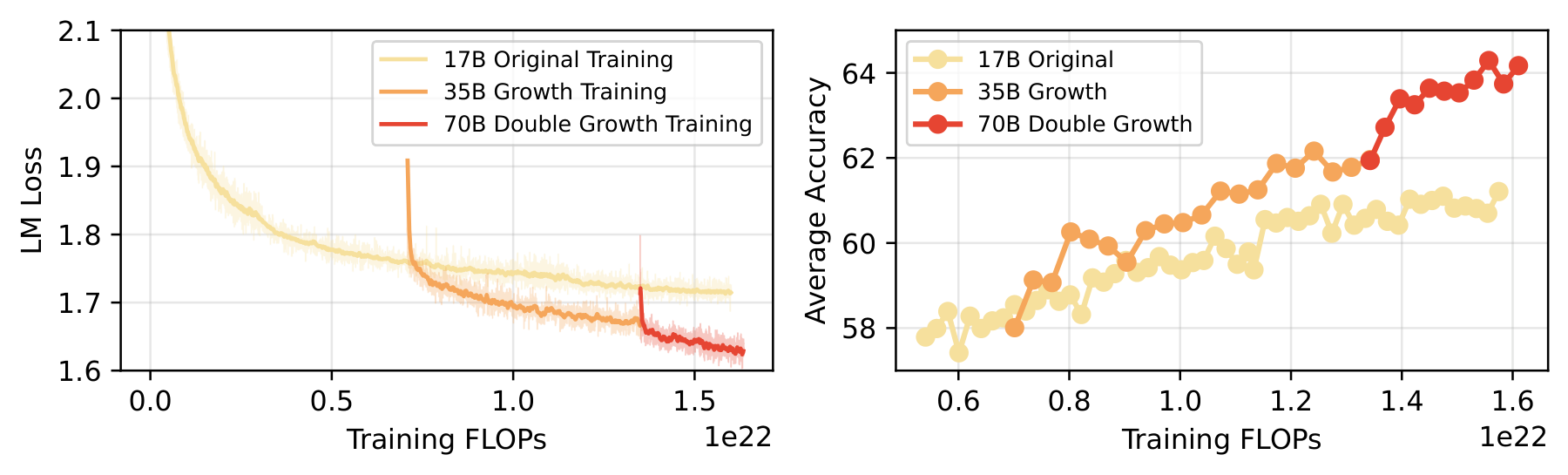 Figure 13. End-to-end training trajectory for the full 17B→35B→70B pipeline over 1 trillion tokens. Brief loss spikes at each growth event are followed by rapid recovery, with steady accuracy gains throughout.
Interposition’s advantage is equally clear at 17B scale:
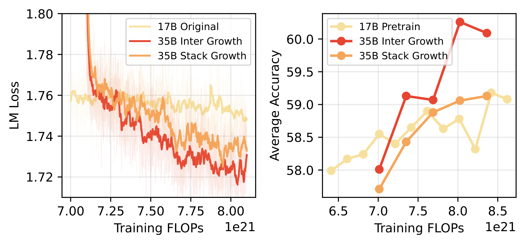 Figure 14. Interposition vs. Stacking at 17B→35B scale. The advantage of Interposition persists and is consistent with findings at 3B scale, validating the generality of the method.
These experiments yield important conclusions:
- vs training from scratch (same extra FLOPs): accuracy is 10.6% higher (64.17 vs 58.55, relative improvement)
- vs 17B base (controlling total FLOPs): accuracy is 4.0% higher (64.17 vs 61.21)
- Growth unlocks the performance ceiling: the 17B model had largely saturated after 600B tokens, but growing to 70B produced a substantial further improvement
- Intermediate models are already strong: growing from 17B to 35B contributes +2.21 accuracy, and subsequently from 35B to 70B adds another +2.21. Each growth step is effective, not just the final one.
Furthermore, our 17B model has been trained for approximately $13 \times F_c$ ($F_c \approx 5.3 \times 10^{20}$), far exceeding the $1 \times F_c$ boundary discussed earlier. This means the model is “deeply converged”—precisely the scenario where Interposition excels.
Final Remarks
The take-away message: don’t throw away your checkpoints. They can be grown into larger models that perform as well as training from scratch, while saving significant GPU resources.
Practical recommendations:
- Use Interposition for depth growth—unless your model has been trained less than $1 \times F_c$ (rare these days)
- Add small noise ($\alpha \approx 0.01$) when duplicating experts
- Prefer checkpoints from the constant-LR phase rather than annealing
- Budget at least 1× the sunk FLOPs for continued training
- Don’t worry about ordering—depth first or width first, they’re orthogonal
For more details and appendix content, please refer to the original paper. Feedback and discussion are welcome!
Paper: arxiv.org/abs/2510.08008v2 Code: github.com/Mr-Philo/Orthogonal-Model-Growth